Creating a Machine Learning Model Using ADLS Gen2

Intro

Azure Data Lake Storage Gen2 is a new version of the storage solution available on Azure cloud platform. It mixes the best features of both Azure Data Lake Storage Gen1 and Azure Storage. Azure Data Lake Storage Gen1 supports hierarchical file system for storing data in directories. It allows implementing some features for both file and directory levels. For example, you can specify the security settings for all files in a directory as well as for the single file in a directory. Azure Storage has a flat namespace for storing objects (binary large objects - blobs). Azure Data Lake Storage Gen2 uses the file system for analytics, but it manages to support a high level of scalability and cost-efficiency which are peculiar to Azure Storage.

In this tutorial, we will demonstrate how to create ADLS Gen2 instance in your Azure account, how to set it up, and how to load the data into prepared storage. Then, we will connect Dremio to ADLS Gen2 to load the data into Dremio workspace. After the connection, the data will be curated using Dremio tools. During the curation, we are going not only to perform some basic data preparation for the further machine learning model creation. We also want to show interesting tricks which are not required by our current case but may be useful in your work with Dremio.

The data we will use is the Energy efficiency data set. It includes information about different building’s parameters and energy efficiency requirements, which is expressed in the heating load and cooling load requirements of buildings. We want to build a machine learning model which would be able to predict the target variables based on the building features (for example, surface area, wall area, roof area, overall height, orientation, etc.). As both heating and cooling load are the real continuous numbers, the task we need to solve is a regression. So, we will use machine learning algorithms suitable specifically for this type of tasks. To make the data curation process in Dremio more complicated and interesting, we have intentionally split the data into 2 chunks and load them to the ADLS Gen2 separately in order to join them later in Dremio.

Assumptions

We assume that you have the next instruments already installed on your local system:

• Dremio 3.2
• Azure account
• Python 3.6
• Pyodbc
• Dremio ODBC Driver
• Python packages: pandas, scikit-learn, plotly express
• Jupyter Notebook environment
• Ubuntu OS

The aforementioned list includes the recommended tools which should allow you to follow actions in our tutorial in the most similar way to how we describe those actions. Nevertheless, it is not mandatory to have exactly the same set of tools.

Preparation steps

First what we need to do is to set up Azure Data Lake Storage Gen2 account and load the data.

Prior to the storage instance creation, we have to create a resource group, with which the ADLS Gen2 will be associated. So, log in to your Azure account using the Azure portal and click on the Resource groups button in the left-side menu. Then, click Add:

The window for a new resource group creation should appear:

There you should specify the name of the resource group you want to create (we chose energy_efficiency name), select the subscription plan you are going to use and the region with which this resource group will be associated. Then click the Review + Create button. On the next tab you will see the summary of the resource group you are creating:

If everything is OK, you can confirm the creation by pressing Create. Now, when you go to the resource groups section, you should see the created resource group in the list of groups. This means that the creation was completed successfully and you are ready to go to the next step - storage account creation.

Go to All services tab in the left-side menu. Then, select Storage and click on the Storage accounts:

On the storage accounts page click the Add button. The form for a new storage account creation will appear. It consists of two parts. The first part is called Project details. Here you should select the subscription plan and choose the resource group. We pick the resource group which we have created earlier.

The second part is called the Instance details. There we should specify parameters related to our storage instance, which include the name and location as mandatory parameters, and performance, account kind, replication, and access tier as optional parameters. We can leave those parameters with their default options as you can see on the image below. After you finish with form filling, press Next: Advanced > button.

On the Advanced tab, you can leave everything with their default values, but assure that Hierarchical namespace for Data Lake Storage Gen2 is enabled, as on the image below.

Now you can press Review + Create button to generate a summary of the storage account instance you are going to create (see the image below). Check if there are not any mistakes and click Create to finalize the creation process.

If everything is OK, then the storage account deployment process should be completed successfully. You will see the corresponding notification:

As you can see, there is no mention about the fact, that the created storage is ADLS Gen2 storage. To assure that we have created what we intended to, we should click on the storage and check if there is a phrase “Data Lake Gen2 file systems”, like on the image below.

It’s time to upload the data to ADLS Gen2. Prior to uploading our files, we need to create a file system. So, in the menu of the storage account, select File systems. Then, click the + File systems button. You will need to specify the name of the file system (we chose adlsgen2energy). Click OK and the filesystem should be created:

To upload files into storage, we will use the special Azure’s software called Microsoft Azure Storage Explorer. You can get it here for free. After installation, you may have the folder with this software which should look like on the image below. To start the program, you can use the highlighted object:

You will see the loading window, something like this:

Note that it is possible that you will need to install .Net 2.0 Framework, which is a dependency of Microsoft Azure Storage Explorer.

Once you manage to run Storage Explorer, you have to authenticate using the credentials for your Azure account. After logging in, you will be able to see the tree structure of your storage in the left side of the window:

On the next step, find the name of the filesystem you have created earlier (adlsgen2energy in our case):

To upload needed files, you have to select the filesystem and then press the corresponding (upload) button in the Storage Explorer. The file browsing window should appear:

In this window, specify the file you want to upload to the storage. In our case, we uploaded 2 files successfully: energy_first.csv and energy_second.csv.

Now, the preparation process is finished, and we can connect ADLS Gen2 to Dremio.

ADLS Gen2 and Dremio connection

In order to connect storage instance to Dremio, open Dremio GUI in your browser and click on the button for adding a new source. Choose the Azure Storage option in the next window (this is how ADLS Gen2 is denoted in Dremio):

In the next window, we should enter the parameters needed to establish a connection. Among them the name of the source (adlsgen2_energy in our case) and the storage account name (energyeffdremio). Other options, including account kind, we leave in their default state. The very important parameter is the Shared Access Key. You can find it in the Access keys section of your storage account (key1):

The filled New Azure Storage Source window looks like this:

After the successful creation of the connection, you will see the name of the source in the list of sources, as well as you will be able to find the needed data files in the storage’s filesystem:

Now we can start preprocessing our data in Dremio.

Data curation in Dremio

We will start data preprocessing by joining two separate tables: energy_first and energy_second. This could be done from any dataset. Press the Join button in the upper menu. Then, select another table with which you want to join the current table. As a next step, you need to specify columns (outer keys) which should be used to perform join:

After joining, we don’t need to have index columns in our dataset, so we want to drop them:

As a result, we obtained the following dataset:

You can see that the first row in this dataset is actually the name of the columns. So, we want to rename all the columns:

After renaming, we don’t need to have the first row at all. So, we click on the Exclude… button in the dropdown menu called from the first column (X1). In the next window, we select the value we want to exclude (X1).

After applying, the entire first row will be removed from the dataset.

You can notice that our numeric values are saved as strings. If you will try to convert datatype to float (by clicking on Abc symbols and selecting Float), you will see an error. This is because the values have comma instead of point as an integer and float parts separator. So, we need to transform values. Here is how we did this:

We click Calculated Field… button near the name of the column. Then, we enter a formula which takes a certain number of characters from the left side of each string value, a certain number of characters from the right side, and concatenate both parts using point (“.”). After that, we can successfully apply type conversion operation:

We can perform this sequence of actions for each column in our dataset.

The calculated field is very useful feature Dremio supports. For example, it can be useful for feature engineering in Data Science, when you need to create a new column based on some existing columns. Look at the image below. There we create a new column named X1X2* and the values for this column are calculated as the result from multiplying column 1 and column 2 (so, X1 feature and X2 feature).

Now our data preprocessing work is done, and we should save the curated dataset in the adls_energy_space workspace. To do this, we should Click Save As… and select the workspace where we want to store the curated dataframe.

Regression machine learning model creation

We have 2 target variables: Y1 (heating load) and Y2 (cooling load). That’s why we need to build 2 separate models, the first for predicting Y1, and the second for Y2. As we stated in the assumptions section, all our code we are writing and executing in the Jupyter Notebook. At the beginning of the notebook, we import some needed libraries:

import pandas as pd
import numpy as np
import pyodbc
from sklearn.metrics import mean_squared_error
from sklearn.metrics import r2_score
from sklearn.model_selection import train_test_split
import plotly_express as px

After that, we connect to Dremio to get curated data. Notice how we specify host, port, username, and password for Dremio account. Also, we use SQL query to fetch data from Dremio.

host='localhost'
port=31010
uid ='username'
pwd = 'password'
driver = '/opt/dremio-odbc/lib64/libdrillodbc_sb64.so'
cnxn = pyodbc.connect("Driver={};ConnectionType=Direct;HOST={};PORT={};AuthenticationType=Plain;UID={};PWD={}".format(driver,host,port,uid,pwd),autocommit=True)
sql = "SELECT * FROM adls_energy_space.energy_curated"
df = pd.read_sql(sql,cnxn)

Here is a sample of the imported data:

The shape of our dataframe is (768, 10). So, this is a small dataset. Nevertheless, we hope that it should be enough to build good predictive models.

Now, we want to perform some exploratory data analysis (EDA) to understand the data better. We want to start by displaying some basic statistics about the dataset:

We can see that different features are distributed in different ranges. For example, the X8 feature has values from 0 to 5, while the X2 is distributed in the range from 514 to 808. This could be bad for some metrics algorithms, leading to slow training or even worse results. So, we decided to perform feature scaling later. Feature scaling will transform the dataset to the state where all features lay in a similar range of values, for example, from 0 to 1. In the same way, the relationships between values remain the same, so no information is lost.

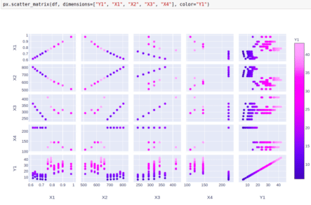
Let’s use Plotly Express library to draw some visualizations. Firstly, we want to look at the correlation between different features as well as between features and target variables. On the image below we visualize the relationships between Y1, X1, X2, X3, and X4.

On the next image, we consider Y1, X5, X6, X7, and X8.

The picture for Y2 is pretty much the same. It is obvious, that the relationships between target variables and features are not very complex.

What we also want to look at is the distributions of the target variables. Here is the histogram of Y1 distribution:

And here is the distribution of the Y2 variable:

We can see that the distributions of Y1 and Y2 are pretty similar.

Now, we can start working directly on the machine learning model creation, which will predict the target variable. To start, we separate the features (X) and target variable (y). Then, we split the dataset into training and testing subsets.

X = df.drop(columns=['Y1', 'Y2'])
y = df['Y1']
X_train, X_test, y_train, y_test = train_test_split(X, y, test_size=0.2, random_state=42)

The next thing we need to do is feature scaling, which we have mentioned earlier.

from sklearn.preprocessing import MinMaxScaler
scaler = MinMaxScaler()
X_train_scaled = pd.DataFrame(data=scaler.fit_transform(X_train),
                         columns=['X1', 'X2', 'X3', 'X4', 'X5', 'X6', 'X7', 'X8'])
X_test_scaled = pd.DataFrame(data=scaler.transform(X_test),
                         columns=['X1', 'X2', 'X3', 'X4', 'X5', 'X6', 'X7', 'X8'])

There are a couple of very important things you need to understand about feature scaling. First, you have to perform it after splitting into training and testing sets. This should be done in order to avoid so-called data leakage. Your model shouldn’t know anything about the new data (testing dataset) at the time of training. Instead, when you perform feature scaling on a whole dataset, you include some sort of information about the distribution of testing set in the training set. So, it is necessary to perform feature scaling independently for training and testing dataset.

The second important thing is the way how to perform feature scaling. There are several methods of scaling, but all use some meta information about the data. For example, we are using MinMaxScaler. This scaler creates a reflection of data on the range from 0 to 1, where the minimum value of the original data transforms into 0 and the maximum value transforms into 1. So, the minimum and maximum values are meta information used by scaler to perform scaling. We need to get these values from the training dataset and use them for scaling testing dataset as well, regardless of the minimum and maximum values that are presented in the testing dataset. In our code, this idea is realized through calling method fit_transform() on the X_train set, and by calling transform() method on the X_test set.

Let’s look at the scaled training dataset:

We can see that now all features lie in the range from 0 to 1.

Now, we import the needed regression algorithms. We want to train such models as ordinary linear regression, support vector machines, K nearest neighbors, random forest, gradient boosting, and simple neural network.

from sklearn.linear_model import LinearRegression
from sklearn.svm import SVR
from sklearn.neighbors import KNeighborsRegressor
from sklearn.ensemble import RandomForestRegressor
from sklearn.ensemble import GradientBoostingRegressor
from sklearn.neural_network import MLPRegressor

We will evaluate models performance using 2 metrics: square root from the mean squared error and R2-score (coefficient of determination). The first metric indicates the average error (the difference between true and predicted value) which our model makes on the testing dataset. The second metric shows the percent of the variance of the target variable which the model managed to explain using independent variables (features). The best value for the square root from the mean squared error is 0 because this means that there is no error. The best value for R2-score is 1 meaning that absolutely all variance is explained by the model.

Let’s start from simple linear regression:

We can see that the linear model works well enough on this data: it explains around 91% of the variance and the average error is around 3. Remember that our target variable (Y1) vary from 6 to 43. On this range, the error equal to 3 can be considered as a rather low error. Let’s now train and evaluate all other models and compare results.

We can see, that all models are better than simple linear regression. For some models, we needed to tune hyperparameters (like* C, n_neighbors, n_estimators, learning_rate, hidden_layer_sized*) to improve results. One of the main tasks of these hyperparameters is to control the balance between overfitting and underfitting (bias-variance tradeoff). The best model is gradient boosting. It makes an average error of less than 0.5, which is very good in our case. Also, it explains more than 99% of the variance in the target variable. At the same time, to achieve these results we had to tune hyperparameters in a way, which led to the very slow training process. On the other hand, the results of the random forest regressor are only slightly worse. This difference is not even material. The training process was very fast. So, taking into account these facts, we can make the conclusion that the random forest algorithm is the best model for this task and this data.

The neural network is a very powerful tool. Nevertheless, we can see that in our case it is not the best choice. This is probably because of the small amount of data. Neural networks require a lot of data to work well. Also, as we could see during EDA step, the relations between the target variable and features are not very complex. There is an experts’ opinion that neural networks should be applied to very complex problems. In those cases, they can demonstrate all their strengths.

Let’s now perform the same steps for Y2.

Splitting into training and test set:

X = df.drop(columns=['Y1', 'Y2'])
y = df['Y2']
X_train, X_test, y_train, y_test = train_test_split(X, y, test_size=0.2, random_state=42)

Feature scaling:

scaler = MinMaxScaler()
X_train_scaled = pd.DataFrame(data=scaler.fit_transform(X_train),
                         columns=['X1', 'X2', 'X3', 'X4', 'X5', 'X6', 'X7', 'X8'])
X_test_scaled = pd.DataFrame(data=scaler.transform(X_test),
                         columns=['X1', 'X2', 'X3', 'X4', 'X5', 'X6', 'X7', 'X8'])
Linear regression, support vector machines, and K nearest neighbors algorithms:

Random forest, gradient boosting, and neural network models:

We can see that in general, the results for the variable Y2 are worse than for Y1. So, it is harder for the models to predict the cooling load than to predict the heating load. Also, an interesting thing here is that gradient boosting performs considerably better than random forest.

Conclusion

In this tutorial, we showed how to create and set up ADLS Gen2, how to load data in that storage, and how to connect it to Dremio. Then, we performed initial data preprocessing in Dremio, which included tables joining, rows and columns removing, creation of the calculated fields, type conversions. After the data curation was finished, we imported that data to Python script, which we have written in Jupyter Notebook. Using the Python programming language and its libraries for data science and machine learning, we performed further data preparation, exploratory data analysis, and have created a range of machine learning models for regression task. The best results we got using gradient boosting and random forest algorithms. These models could be used to predict the heating and cooling load of the building based on its features.

We hope you enjoyed this tutorial, checkout the rest of our tutorials and resources page to learn more about how you can gaining insights from your Azure data, faster, using Dremio.