Introduction to Apache Iceberg Using Spark

Note: You can find this and many other great Apache Iceberg instructional videos and articles at our Apache Iceberg 101 article.

Apache Iceberg is an open table format that enables robust, affordable, and quick analytics on the data lakehouse and is poised to change the data industry in ways we can only begin to imagine. Check out this webinar recording to learn about the features and architecture of Apache Iceberg. In this article, we get hands-on with Apache Iceberg to see many of its features and utilities available from Spark. 

Other Hands-On Apache Iceberg Exercises:

• Intro to Dremio, Nessie, and Apache Iceberg on Your Laptop
• From SQLServer -> Apache Iceberg -> BI Dashboard
• From MongoDB -> Apache Iceberg -> BI Dashboard
• From Postgres -> Apache Iceberg -> BI Dashboard
• From MySQL -> Apache Iceberg -> BI Dashboard
• From Elasticsearch -> Apache Iceberg -> BI Dashboard
• From Kafka -> Apache Iceberg -> Dremio

Apache Iceberg 101

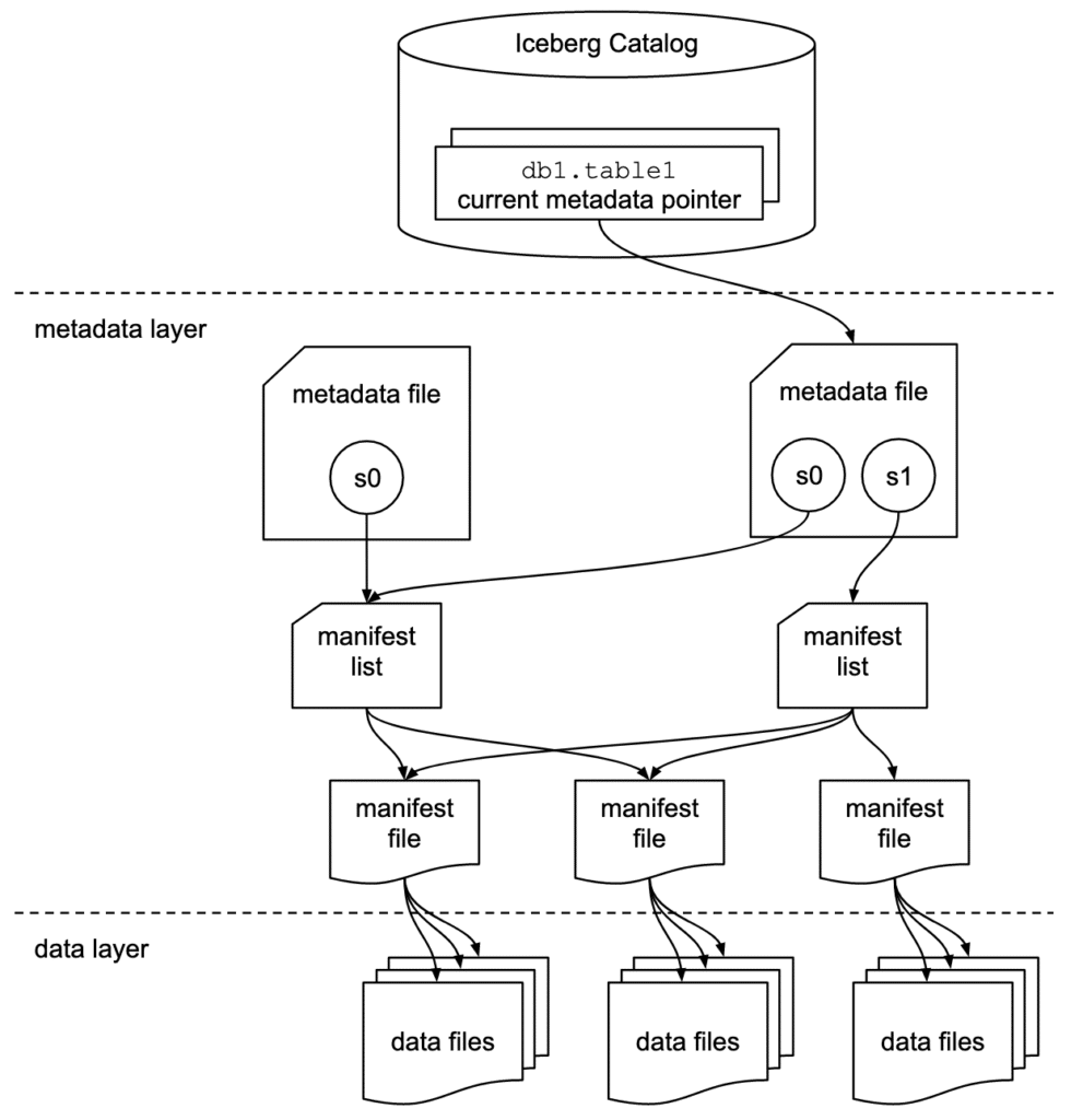
Apache Iceberg has a tiered metadata structure which is key to how Iceberg provides high-speed queries for both reads and writes. The following summarizes the structure of Apache Iceberg to see how this works. If you are already familiar with Iceberg’s architecture, then feel free to skip ahead to “Getting Hands-On with Apache Iceberg.”

Data Layer

Starting from the bottom of the diagram, the data layer holds the actual data in the table, which is made up of two types of files: 

Data files – Stores the data in file formats such as Parquet or ORC. 

Delete files – Tracks records that still exist in the data files, but that should be considered as deleted.

Metadata Layer

Apache Iceberg uses three tiers of metadata files which cover three different scopes:

Manifest files – A subset of the snapshot, these files track the individual files in the data layer in the subset along with metadata for further pruning. 

Manifest lists – Defines a snapshot of the table and lists all the manifest files that make up that snapshot with metadata on the manifest files for pruning.

Metadata files – Defines the table and tracks manifest lists, current and previous snapshots, schemas, and partition schemes.

The Catalog

The catalog tracks a reference/pointer to the current metadata file. This is usually some store that can provide some transactional guarantees like a relational database (Postgres, etc.) or metastore (Hive, Project Nessie, Glue).

Getting Hands-On with Apache Iceberg

Prerequisite: You must have Docker installed. If you don’t, you can download and install it here.

So let’s take Apache Iceberg for a test drive together. To keep things as simple as possible, we use this self-contained Docker container which has everything you need:

docker pull alexmerced/spark3-3-iceberg0-14

We then open up the container in interactive mode.

docker run --name iceberg-sandbox -it 
alexmerced/spark3-3-iceberg0-14

An Iceberg-enabled engine is the easiest way to use Iceberg. For this example, we  use Spark 3. You can see how to use Apache Iceberg with different engines and platforms on the Apache Iceberg website. This Docker container comes with a simple command to open up SparkSQL configured for Iceberg:

iceberg-init

This command is a custom alias for the following command that opens the SparkSQL shell with Apache Iceberg ready to go:

spark-sql --packages 
org.apache.iceberg:iceberg-spark-runtime-3.3_2.12:0.14.0
    --conf 
spark.sql.extensions=org.apache.iceberg.spark.extensions.Iceberg
SparkSessionExtensions 
    --conf 
spark.sql.catalog.spark_catalog=org.apache.iceberg.spark.SparkSessionCatalog 
    --conf spark.sql.catalog.spark_catalog.type=hive 
    --conf 
spark.sql.catalog.iceberg=org.apache.iceberg.spark.SparkCatalog 
    --conf spark.sql.catalog.iceberg.type=hadoop 
    --conf spark.sql.catalog.iceberg.warehouse=$PWD/warehouse

Let’s break down what each of these flags are doing.

--packages 
org.apache.iceberg:iceberg-spark-runtime-3.3_2.12:0.14.0

This flag is instructing Spark to use the Apache Iceberg package; you want to make sure it’s the right package for the version of Spark and version of Iceberg you plan on using. (You can also just drop the right Iceberg JAR in the Spark JARS folder as well).

    --conf spark.sql.catalog.spark_catalog=org.apache.Apache 
Iceberg.spark.SparkSessionCatalog 
    --conf spark.sql.catalog.spark_catalog.type=hive 
    --conf spark.sql.catalog.iceberg=org.apache.Apache
Iceberg.spark.SparkCatalog 
    --conf spark.sql.catalog.iceberg.type=hadoop 
    --conf spark.sql.catalog.iceberg.warehouse=$PWD/warehouse

This flag creates an Apache Iceberg catalog called “local” whose tables are saved in a directory called “warehouse” in our current working directory.

Now that we have SparkSQL open let’s create a table using Apache Iceberg with the following command:

CREATE TABLE iceberg.db.my_table (name string, age int) USING iceberg;

Now that the table exists, let’s add some data.

INSERT INTO iceberg.db.my_table VALUES ('Bob', 20), ('Steve', 36), ('Fiona', 25), ('Roger', 25);

Now let’s update a record.

UPDATE iceberg.db.my_table SET name='Alex' WHERE name='Steve';

Let’s also update the table schema.

ALTER TABLE iceberg.db.my_table ADD COLUMNS (email string);

Now add another record.

INSERT INTO iceberg.db.my_table VALUES ('John', 56, '[email protected]');

Now let’s query our data.

SELECT * FROM iceberg.db.my_table;

We can now see all the records we created. This may all seem pretty easy, like you’re working with a normal run-of-the-mill transactional database, and that’s the beauty of it. With Apache Iceberg tables we extend our ability to query data as well as to insert, update, delete and modify schemas on large distributed datasets quickly and safely across engines and file formats.

If we wanted to create an Iceberg table from an existing source, we would just create a view from the source data and then use a CTAS (Create Table AS) to create an Iceberg table from that view. (Learn more about migrating data into Iceberg and try this Iceberg migration exercise.)

As an example, in the Docker container, there is a sample file in ~/sampledata/Woorker_Coop.csv. To create a SQL View from this data, we simply enter the following command:

CREATE TEMPORARY VIEW my_data
USING csv
OPTIONS (
  path 'sampledata/Worker_Coops.csv',
  header true,
  inferSchema true
);

Then we can take that view and use a CTAS statement to create an Iceberg table from it.

CREATE TABLE iceberg.db.worker_coop
USING iceberg
PARTITIONED BY (Borough)
AS (SELECT * FROM my_data ORDER BY Borough ASC);

(Note: Notice that we partitioned the table Borough; there are a lot of really cool ways we can optimize the table with partitioning which are enhanced with Iceberg features like hidden partitioning and partition evolution.)

Now you know how to create tables from scratch and from sources like data files and other existing tables using a CTAS.

Now let’s run a few DML transactions on this new table before inspecting the table under the hood.

Let’s delete all entries from the Bronx.

DELETE FROM iceberg.db.worker_coop 
WHERE Borough = 'BRONX';

Now update all Staten Island entries to Richmond County.

UPDATE iceberg.db.worker_coop 
SET Borough = 'RICHMOND COUNTY' 
WHERE Borough = 'STATEN IS';

Inspecting Our Table

We can view a lot of information about our table using the Iceberg SQL extensions. Here are  a few examples.

We can inspect our table's history:

SELECT * FROM iceberg.db.worker_coop.history;

We can inspect our table's snapshots:

SELECT * FROM iceberg.db.worker_coop.snapshots;

We can inspect our table's files:

• Notice in the output when looking at the file paths we can see that the folders are organized by the partitioning scheme we chose.

SELECT file_path FROM iceberg.db.worker_coop.files;

We can inspect our table's manifests:

SELECT path, partition_spec_id FROM iceberg.db.worker_coop.manifests;

We can inspect our table's partitions:

SELECT partition, spec_id FROM iceberg.db.worker_coop.partitions;

Looking Under The Hood

Now let’s take a look at what Apache Iceberg created when we ran all that SQL. First, let’s quit SparkSQL by running exit;. Next, change directories into my_table which is inside a db folder that is inside that warehouse folder we created earlier.

cd warehouse/db/my_table

If you look inside this folder,  notice two folders: data and metadata. Let’s look at their contents.

Data

ls data

This should display several Parquet files which represent our data at several different points.

00000-0-9b380798-8d30-46c1-b518-54f74ca5b2c6-00001.parquet
00000-8-d14d9687-cc70-44a0-b2d5-d32917d7aab5-00001.parquet
00002-2-ffe0fa9a-1a3d-4dfa-aa8e-f8931eeecec7-00001.parquet
00000-6-71b79309-da32-441a-8751-e52522c89287-00001.parquet
00001-1-e6bc34d1-ae7d-4c18-b5af-d5925034b8fb-00001.parquet
00003-3-b1c850ba-b2f8-42ea-ae63-2390a803b42b-00001.parquet

To explore the contents of these files install PyArrow (Python required).

pip install pyarrow

Open the Python shell.

python3

Import pyarrow.parquet.

import pyarrow.parquet as pq

Create a dataframe from the file and save it in a variable (make sure you use the file name on your system which should be different than below).

table1 = 
pq.read_table("data/00000-0-9b380798-8d30-46c1-b518-54f74ca5b2c6-00001.parquet")

Print the dataframe to see the contents, which should be some of the data from your table.

print(table1)

Exit the Python shell.

exit()

Metadata

ls metadata

This should display Avro and JSON files which are the metadata that tracks our table’s different snapshots, schema changes, etc.

098a1061-a281-4260-94d3-6f2d69a4bdd1-m0.avro
adae77ab-683e-41af-b9f2-b790a297db81-m0.avro
snap-5137078496018731240-1-3232cbec-a1ef-4e70-b944-03fe14f95ca0.avro  v3.metadata.json  version-hint.text
3232cbec-a1ef-4e70-b944-03fe14f95ca0-m0.avro
snap-3749518827480390728-1-098a1061-a281-4260-94d3-6f2d69a4bdd1.avro  v1.metadata.json           v4.metadata.json
3232cbec-a1ef-4e70-b944-03fe14f95ca0-m1.avro
snap-5061571068301453651-1-adae77ab-683e-41af-b9f2-b790a297db81.avro  v2.metadata.json           v5.metadata.json

Let’s take a look at the most recent metadata file, which for this example is V5.

cat metadata/v5.metadata.json

Or,

less metadata/v5.metadata.json

You can see this large JSON object with data about our table. Let's review a few of the fields that enable some of Apache Iceberg’s features.

  "schema" : {
    "type" : "struct",
    "schema-id" : 1,
    "fields" : [ {
      "id" : 1,
      "name" : "name",
      "required" : false,
      "type" : "string"
    }, {
      "id" : 2,
      "name" : "age",
      "required" : false,
      "type" : "int"
    }, {
      "id" : 3,
      "name" : "email",
      "required" : false,
      "type" : "string"
    } ]
  },
  "current-schema-id" : 1,
  "schemas" : [ {
    "type" : "struct",
    "schema-id" : 0,
    "fields" : [ {
      "id" : 1,
      "name" : "name",
      "required" : false,
      "type" : "string"
    }, {
      "id" : 2,
      "name" : "age",
      "required" : false,
      "type" : "int"
    } ]
  }, {
    "type" : "struct",
    "schema-id" : 1,
    "fields" : [ {
      "id" : 1,
      "name" : "name",
      "required" : false,
      "type" : "string"
    }, {
      "id" : 2,
      "name" : "age",
      "required" : false,
      "type" : "int"
    }, {
      "id" : 3,
      "name" : "email",
      "required" : false,
      "type" : "string"
    } ]
  } ],

This section tracks our current and past schemas. You can see that the current schema array has our old name/age schema followed by our name/age/email schema.

 "partition-spec" : [ ],
  "default-spec-id" : 0,
  "partition-specs" : [ {
    "spec-id" : 0,
    "fields" : [ ]
  } ],
  "last-partition-id" : 999,

This is where any partitioning details would be included, however, we did not specify any partitions when we created our table but we could have done so by adding a PARTITIONED BY clause to our CREATE TABLE statement like the following (assuming we had a born_at date field):

CREATE TABLE iceberg.db.my_table (name string, age int) USING iceberg PARTITIONED BY (hour(born_at));

Since our partitioning scheme is just something tracked in the metadata, repartitioning the data or querying data in ways that it isn’t partitioned (example: query of a day for data partitioned by the hour) is basically free versus partitioning by directory.

  "current-snapshot-id" : 3749518827480390728,
  "snapshots" : [ {
    "snapshot-id" : 5061571068301453651,
    "timestamp-ms" : 1639695247304,
    "summary" : {
      "operation" : "append",
      "spark.app.id" : "local-1639692458952",
      "added-data-files" : "4",
      "added-records" : "4",
      "added-files-size" : "2586",
      "changed-partition-count" : "1",
      "total-records" : "4",
      "total-files-size" : "2586",
      "total-data-files" : "4",
      "total-delete-files" : "0",
      "total-position-deletes" : "0",
      "total-equality-deletes" : "0"
    },
    "manifest-list" : "/home/docker/warehouse/db/my_table/metadata/snap-5061571068301453651-1-adae77ab-683e-41af-b9f2-b790a297db81.avro",
    "schema-id" : 0
  }, {
    "snapshot-id" : 5137078496018731240,
    "parent-snapshot-id" : 5061571068301453651,
    "timestamp-ms" : 1639695651205,
    "summary" : {
      "operation" : "overwrite",
      "spark.app.id" : "local-1639692458952",
      "added-data-files" : "1",
      "deleted-data-files" : "1",
      "added-records" : "1",
      "deleted-records" : "1",
      "added-files-size" : "656",
      "removed-files-size" : "650",
      "changed-partition-count" : "1",
      "total-records" : "4",
      "total-files-size" : "2592",
      "total-data-files" : "4",
      "total-delete-files" : "0",
      "total-position-deletes" : "0",
      "total-equality-deletes" : "0"
    },
    "manifest-list" : "/home/docker/warehouse/db/my_table/metadata/snap-5137078496018731240-1-3232cbec-a1ef-4e70-b944-03fe14f95ca0.avro",
    "schema-id" : 0
  }, {
    "snapshot-id" : 3749518827480390728,
    "parent-snapshot-id" : 5137078496018731240,
    "timestamp-ms" : 1639696657970,
    "summary" : {
      "operation" : "append",
      "spark.app.id" : "local-1639692458952",
      "added-data-files" : "1",
      "added-records" : "1",
      "added-files-size" : "970",
      "changed-partition-count" : "1",
      "total-records" : "5",
      "total-files-size" : "3562",
      "total-data-files" : "5",
      "total-delete-files" : "0",
      "total-position-deletes" : "0",
      "total-equality-deletes" : "0"
    },
    "manifest-list" : "/home/docker/warehouse/db/my_table/metadata/snap-3749518827480390728-1-098a1061-a281-4260-94d3-6f2d69a4bdd1.avro",
    "schema-id" : 1
  } ],

This section shows our current snapshot which points to the manifest list that covers the current snapshot. After the current snapshot, there is an array of snapshots, which is what enables time travel. Having a reference to all previous snapshots allows you to refer to previous points in time and query the data as it was in that snapshot.

This process may beg the question of required maintenance as you accumulate files representing your data at different points. There are recommended patterns for maintaining Iceberg tables such as expiring snapshots, deleting orphan files, and compaction which all have built-in settings that make them easy to carry out.

Conclusion

You’ve had the opportunity to create and edit an Apache Iceberg table and can see how easy it can be. Using Apache Iceberg tables, you can  unlock the speed and flexibility that was not possible before across different file types and engines. Apache Iceberg makes using open data architecture quite compelling. 

Apache Iceberg tables can also be easily used with the Dremio Cloud platform. With Dremio Sonar you can efficiently query Iceberg tables and Dremio Arctic can serve as your Iceberg catalog, enabling git-like semantics (branching/merging) when working with Iceberg tables. You can also explore the structure of Apache Iceberg tables using Dremio.

You can learn more about Apache Iceberg tables at Subsurface, the open lakehouse community resource page, and see how to use Apache Iceberg with your data lakehouse with Dremio as well as how to make Iceberg tables using AWS Glue.