63 minute read · June 25, 2021
Apache Iceberg: An Architectural Look Under the Covers
· Director of Technical Advocacy, Dremio
If you prefer videos over written text, here’s a recording of a presentation of this content
Introduction
Data lakes have been built with a desire to democratize data — to allow more and more people, tools, and applications to make use of more and more data. A key capability needed to achieve this is hiding the complexity of underlying data structures and physical data storage from users. The de facto standard to achieve this has been the Hive table format, released by Facebook in 2009 that addresses some of these problems, but falls short at data, user, and application scale. So what is the answer? Apache Iceberg.

In this article, we’ll go through:
- The definition of a table format, since the concept of a table format has traditionally been embedded under the “Hive” umbrella and implicit
- Details of the long-time de facto standard, the Hive table format, including the pros and cons of it. We’ll see how these problems created the need for the definition of an entirely new table format
- How the Apache Iceberg table format was created as a result of this need. We will also delve into the architectural structure of an Iceberg table, including from the specification point of view and a step-by-step look under the covers of what happens in an Iceberg table as Create, Read, Update, and Delete (CRUD) operations are performed
- Finally, we’ll show how this architecture enables the resulting benefits of this design
What’s a Table Format?
A good way to define a table format is a way to organize a dataset’s files to present them as a single “table”.
Another somewhat simpler definition from a user’s perspective is a way to answer the question “what data is in this table?”.
A single answer to that question allows multiple people, groups, and tools to interact with data in the table at the same time, whether they’re writing to the table or reading from the table.
The primary goal of a table format is to provide the abstraction of a table to people and tools and allow them to efficiently interact with that table’s underlying data.
Table formats are nothing new — they’ve been around since System R, Multics, and Oracle first implemented Edgar Codd’s relational model, although “table format” wasn’t the term used at the time. These systems provided users the ability to refer to a set of data as a table. The database engine owned and managed laying the dataset’s bytes out on disk in the form of files, and addressed the complications that arose, such as the need for transactions.
All interaction with the underlying data, like writing it and reading it, was handled by the database’s storage engine. No other engine could interact with the files directly without corrupting the system. This worked fine for a quite a while. But in today’s big data world where traditional RDBMSs don’t cut it, a single closed engine managing all access to the underlying data isn’t feasible.
With That Simple of a Concept, Why Do We Need a New One?
The big data community has learned over time that when trying to meet business requirements at data, user, and application scale, there are a lot of considerations when it comes to presenting datasets as tables for users and tools.
Some of the challenges encountered were old ones — ones that RDBMSs had already encountered and solved, but were arising again due to the different technologies that had to be used when RDBMSs couldn’t meet key requirements of the big data world. But, the business requirements driving the challenges hadn’t changed.
Some of the challenges encountered were new ones, due to the differences in technologies and scale in the big data world.
To explain why we truly need a new table format, let’s take a look at how the traditionally de facto standard table format came to be, the challenges it has faced, and what solutions were attempted to address these challenges.
How Did We Get Here? A Brief History
In 2009, Facebook realized that while Hadoop addressed many of their requirements such as scale and cost-efficiency, it also had shortcomings they needed to address when it came to improving democratization of their data to the many users who weren’t technical experts:
- Any user who wanted to use the data had to figure out how to fit their question into the MapReduce programming model and then write Java code to implement it.
- There was no metadata defining information about the dataset, like its schema.

To get data in the hands of more of their users and address these shortcomings, they built Hive.
To address problem #1, they realized they needed to provide access in a more general-purpose programming model and language that people were familiar with — SQL. They would build Hive to take a user’s SQL query and translate it for them into MapReduce jobs so that they could get their answers.
A requirement arising out of the solution to #1 as well as to address problem #2, was the need to define what a dataset’s schema was and how to refer to that dataset as a table in a user’s SQL query.
To address the second requirement, the Hive table format was defined (via just 3 bullet points in a white paper and the Java implementation) and has been the de facto standard ever since.
Let’s take a closer look at the Hive table format, a relational layer on top of data lakes designed to democratize analytics to non-technical-experts at scale.
The Hive Table Format
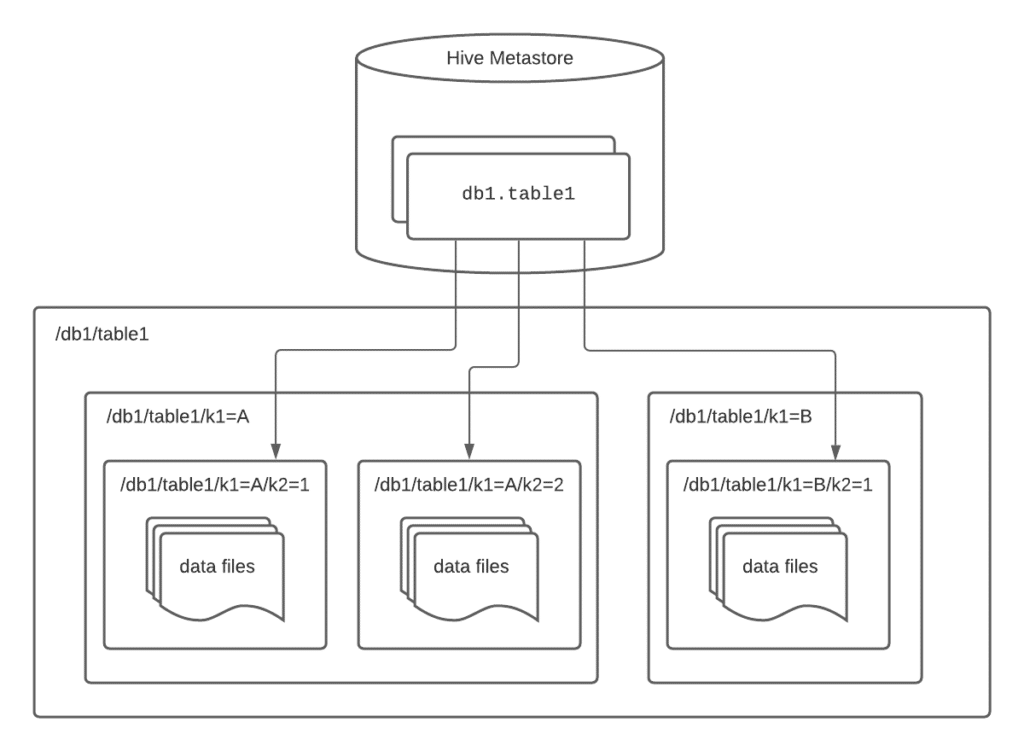
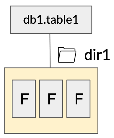
In the Hive table format, a table is defined as the entire contents of one or more directories — i.e., effectively an ls of one or more directories. For non-partitioned tables, this is a single directory. For partitioned tables, which are much more common in the real world, the table is composed of many directories — one directory per partition.
The data making up the table is tracked at the directory level and this tracking is done in the Hive metastore. Partition values are defined via a directory path, in the form /path/to/table/partition_column=partition_value.
Below is an example architecture diagram of a Hive table partitioned by columns k1 and k2.
Pros
Given its status as the de facto standard for the past 10 years or so, the Hive table format has obviously provided a set of useful capabilities and benefits:
- It ended up working with basically every processing engine because it was the only table format in town — it’s been the de facto standard since broader adoption of big data.
- Over the years, it has evolved and provided mechanisms that allowed Hive tables to deliver more efficient access patterns than doing full-table scans for every query, such as partitions and buckets.
- It was file-format agnostic which allowed companies and communities to develop file formats better suited for analytics (e.g., Parquet, ORC) and did not require transformation prior to making the data available in a Hive table (e.g., Avro, CSV/TSV).
- The Hive metastore, storing tables laid out in the Hive table format, provided a single, central answer to “what data is in this table?” for the whole ecosystem of tools that needed to interact with the table, both on the read side and the write side.
- It provided the ability to atomically change data in the table at the whole-partition level, via an atomic swap in the Hive metastore, and therefore enabled a consistent view of the world.
Cons
However, many issues started getting worse and worse when the Hive table format was used at larger data, user, and application scale:
1. Changes to the data are inefficient
- Because partitions are stored in a transactional store (Hive metastore, which is backed by a relational database), you can add and delete partitions in a transactional manner. However, because tracking of the files is done in a filesystem that doesn’t provide transactional capabilities, you can’t add and delete data at the file level in a transactional way.
- The general workaround is to address this at the partition level by replicating the whole partition to a new location behind the scenes, making the updates/deletes while you’re replicating the partition, then updating the partition’s location in the metastore to be the new location.
- This method is inefficient, especially when your partitions are large, you’re changing a relatively small amount of the data in a partition, and/or you’re making changes frequently.
2. There’s no way to safely change data in multiple partitions as part of one operation
- Because the only transactionally consistent operation you can do to change data is to swap a single partition, you can’t change data in multiple partitions at the same time in a consistent way. Even something as simple as adding a file to two partitions can’t be done in a transactionally consistent way. So, users see an inconsistent view of the world and end up with problems making the right decisions and issues trusting the data.
3. In practice, multiple jobs modifying the same dataset isn’t a safe operation
- There isn’t a well-adopted method in the table format to deal with more than one process/person updating the data at a time. There is one method, but it’s so restrictive and causes issues that really only Hive adheres to it. This leads to either strict controls on who can write and when, which an organization has to define and coordinate themselves, or multiple processes concurrently changing the data leading to data loss because the last write wins.
4. All of the directory listings needed for large tables take a long time
- Because you don’t have a list of what files are in all of your partition directories, you need to go get this list at runtime. Getting the response for all the directory listings you need generally takes a long time.
- Ryan Blue, the creator of Iceberg at Netflix, talks about an example use case where it would take over 9 minutes just to plan the query because of these directory listings.
5. Users have to know the physical layout of the table
- If a table is partitioned by when an event occurred, this is often done via multi-level partitioning — first the event’s year, then the event’s month, then the event’s day, and sometimes lower granularity. But when a user is presented with events, the intuitive way to get the events after a certain point in time looks like
WHERE event_ts >= ‘2021-05-10 12:00:00’. In this situation, the query engine does a full table scan, which takes much much longer than if the available partition pruning was done to limit the data. - This full-table scan happens because there is no mapping from the event’s timestamp as the user knows it (2021-05-10 12:00:00) to the physical partitioning scheme (
year=2021, thenmonth=05, thenday=10). - Instead, all users need to be aware of the partitioning scheme and write their query as
WHERE event_ts >= ‘2021-05-10 12:00:00’ AND event_year >= ‘2021’ AND event_month >= ‘05’ AND (event_day >= ‘10’ OR event_month >= '06')(this partition-pruning query gets even more complicated if you were to look at events after May of 2020 instead).
6. Hive table statistics are usually stale
- Because table statistics are gathered in an asynchronous periodic read job, the statistics are often out of date. Furthermore, because gathering these statistics requires an expensive read job that requires a lot of scanning and computation, these jobs are run infrequently, if ever.
- Because of these two aspects, the table statistics in Hive are usually out of date, if they exist at all, resulting in poor plan choice by optimizers, which has made some engines even disregard any stats in Hive altogether.
7. The filesystem layout has poor performance on cloud object storage
- Any time you’re looking to read some data, cloud object storage (e.g., S3, GCS) architecture dictates those reads should have as many different prefixes as possible, so they get handled by different nodes in cloud object storage. However, since in the Hive table format, all data in a partition has the same prefix and you generally read all of the data in a partition (or at least all of the Parquet/ORC footers in a partition), these all hit the same cloud object storage node, reducing the performance of the read operation.
These Problems Get Amplified at Scale — Time for a New Format Altogether
While the above-mentioned issues exist in smaller environments, they get significantly worse at data, user, and application scale.
As with many other successful projects in big data’s history, it’s often tech companies that hit scale problems first and build tools to resolve them. Then, when other organizations experience these same scale problems, they adopt these tools. Most data-driven organizations are already experiencing or starting to deal with these problems now.
A few years ago, Netflix was hitting these problems and employing the standard workarounds with mixed success. After dealing with these problems for a long time, they realized that there may be a better way than continuing to implement more of these workarounds. So, they took a step back and thought about the problems that were occurring, the causes of these problems, and the best way to solve them.
They realized that more band-aids on the Hive table format was not the solution — a new table format was needed.
So, How Did Netflix Fix These Problems?
Netflix figured out that most of the Hive table format’s problems arose from an aspect of it that may appear fairly minor at first, but ends up having major consequences — data in the table is tracked at the folder level.
Netflix figured out that the key to resolving the major issues arising from Hive’s table format was to instead track the data in the table at the file level.
Rather than a table pointing to a directory or a set of directories, they defined a table as a canonical list of files.
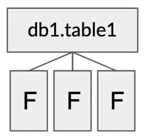
In fact, what they realized was not only could file-level tracking resolve the issues they were hitting with Hive’s table format, it could also lay the foundation for achieving their broader set of analytic goals:
- Provide an always correct and always consistent view of a table
- When making data-driven decisions, those decisions need to be based on trustworthy data. If a report is run while the table is being updated and the report only sees some, but not all, of the changes, that can produce incorrect results, result in wrong or suboptimal decisions, and undermine broader trust in the data within the organization.
- Enable faster query planning and execution
- As mentioned in #4 above, one of Netflix’s use case queries took 9 minutes just to plan the query and just for 1 week’s worth of data. At a minimum, they needed to improve the planning time, as well as overall query execution time to provide an improved user experience and to increase the number of questions a user could ask in order to make more decisions be data-driven.
- Provide users with good response times without them having to know the physical layout of the data
- As mentioned in #5 above, if the user doesn’t query the data in exactly the way the data is partitioned, the query can take much much longer.
- To solve this problem, you can either educate every user and make them do something nonintuitive, but situations like this are almost always better solved in software for user experience and data democratization.
- Enable better and safer table evolution
- Tables change over time with evolving business requirements, additional scale, and additional sources of the data. Since change is inevitable, optimally change management is greatly simplified by the table format so the application layer or data engineering doesn’t need to deal with it.
- If change management is risky, changes don’t happen as often as they need to, and therefore business agility and flexibility is reduced.
- Accomplish all of the goals above at data, user, and application scale
Let’s take a closer look at this new table format, named Iceberg, and how it resolves the problems with Hive’s table format, as well as achieves these broader business and analytic goals.
The Iceberg Table Format
Before diving into the format itself, because “Hive” has been a somewhat nebulous and overloaded term that means different things to different people due to its history, let’s clearly define what Iceberg is and what it isn’t:
| ✅ What Iceberg is | ❌ What Iceberg is not |
| - A table format specification - A set of APIs and libraries for engines to interact with tables following that specification | - A storage engine - An execution engine - A service |
An Iceberg Table’s Architecture
Now, let’s go through the architecture and specification that enables Iceberg to solve the Hive table format’s problems and achieves the goals discussed above by looking under the covers of an Iceberg table.
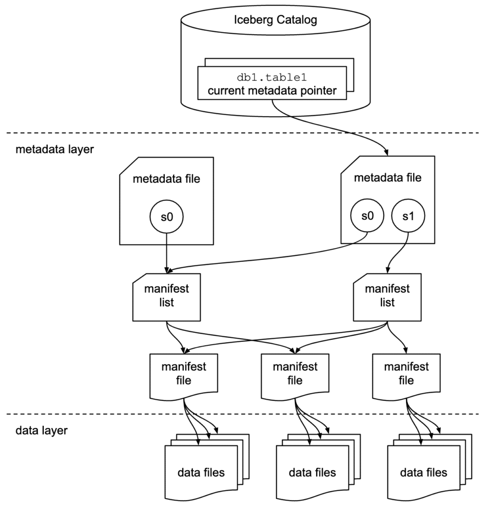
Here’s an architectural diagram of the structure of an Iceberg table:
Iceberg Components
Now, let’s walk through each of the components in the diagram above.
As we walk through them, we’ll also step through the process a SELECT query takes through the components to read the data in an Iceberg table. You’ll see these denoted in boxes below marked with this icon:
There are 3 layers in the architecture of an Iceberg table:
- The Iceberg catalog
- The metadata layer, which contains metadata files, manifest lists, and manifest files
- The data layer
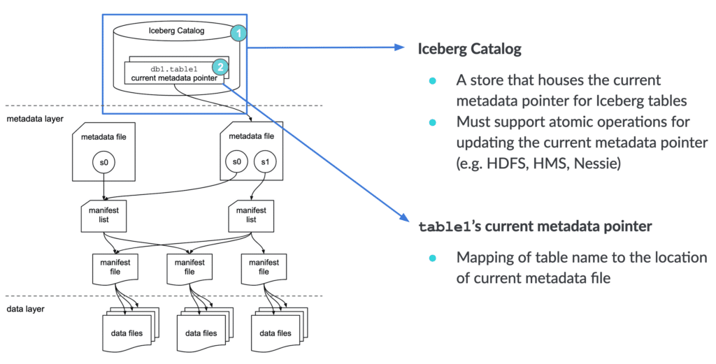
Iceberg catalog
Anyone reading from a table (let alone 10s, 100s, or 1,000s) needs to know where to go first — somewhere they can go to find out where to read/write data for a given table. The first step for anyone looking to read the table is to find the location of the current metadata pointer (note the term “current metadata pointer” is not an official term, but rather a descriptive term because there is no official term at this point and there hasn’t been push-back in the community on it).
This central place where you go to find the current location of the current metadata pointer is the Iceberg catalog.
The primary requirement for an Iceberg catalog is that it must support atomic operations for updating the current metadata pointer (e.g., HDFS, Hive Metastore, Nessie). This is what allows transactions on Iceberg tables to be atomic and provide correctness guarantees.
Within the catalog, there is a reference or pointer for each table to that table’s current metadata file. For example, in the diagram shown above, there are 2 metadata files. The value for the table’s current metadata pointer in the catalog is the location of the metadata file on the right.
What this data looks like is dependent on what Iceberg catalog is being used. A few examples:
- With HDFS as the catalog, there’s a file called
version-hint.textin the table’s metadata folder whose contents is the version number of the current metadata file. - With Hive metastore as the catalog, the table entry in the metastore has a table property which stores the location of the current metadata file.
- With Nessie as the catalog, Nessie stores the location of the current metadata file for the table.

So, when a SELECT query is reading an Iceberg table, the query engine first goes to the Iceberg catalog, then retrieves the entry of the location of the current metadata file for the table it’s looking to read, then opens that file.
Metadata file
As the name implies, metadata files store metadata about a table. This includes information about the table’s schema, partition information, snapshots, and which snapshot is the current one.
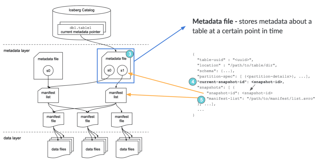
While the above is an abridged sample for illustration purposes, here is an example of the full contents of a metadata file:v3.metadata.json
{
    "format-version" : 1,
    "table-uuid" : "4b96b6e8-9838-48df-a111-ec1ff6422816",
    "location" : "/home/hadoop/warehouse/db2/part_table2",
    "last-updated-ms" : 1611694436618,
    "last-column-id" : 3,
    "schema" : {
        "type" : "struct",
        "fields" : [ {
            "id" : 1,
            "name" : "id",
            "required" : true,
            "type" : "int"
        }, {
            "id" : 2,
            "name" : "ts",
            "required" : false,
            "type" : "timestamptz"
        }, {
            "id" : 3,
            "name" : "message",
            "required" : false,
            "type" : "string"
        } ]
    },
    "partition-spec" : [ {
        "name" : "ts_hour",
        "transform" : "hour",
        "source-id" : 2,
        "field-id" : 1000
    } ],
    "default-spec-id" : 0,
    "partition-specs" : [ {
        "spec-id" : 0,
        "fields" : [ {
            "name" : "ts_hour",
            "transform" : "hour",
            "source-id" : 2,
            "field-id" : 1000
        } ]
    } ],
    "default-sort-order-id" : 0,
    "sort-orders" : [ {
        "order-id" : 0,
        "fields" : [ ]
    } ],
    "properties" : {
        "owner" : "hadoop"
    },
    "current-snapshot-id" : 1257424822184505371,
    "snapshots" : [ {
        "snapshot-id" : 8271497753230544300,
        "timestamp-ms" : 1611694406483,
        "summary" : {
            "operation" : "append",
            "spark.app.id" : "application_1611687743277_0002",
            "added-data-files" : "1",
            "added-records" : "1",
            "added-files-size" : "960",
            "changed-partition-count" : "1",
            "total-records" : "1",
            "total-data-files" : "1",
            "total-delete-files" : "0",
            "total-position-deletes" : "0",
            "total-equality-deletes" : "0"
        },
        "manifest-list" : "/home/hadoop/warehouse/db2/part_table2/metadata/snap-8271497753230544300-1-d8a778f9-ad19-4e9c-88ff-28f49ec939fa.avro"
    },
    {
        "snapshot-id" : 1257424822184505371,
        "parent-snapshot-id" : 8271497753230544300,
        "timestamp-ms" : 1611694436618,
        "summary" : {
            "operation" : "append",
            "spark.app.id" : "application_1611687743277_0002",
            "added-data-files" : "1",
            "added-records" : "1",
            "added-files-size" : "973",
            "changed-partition-count" : "1",
            "total-records" : "2",
            "total-data-files" : "2",
            "total-delete-files" : "0",
            "total-position-deletes" : "0",
            "total-equality-deletes" : "0"
        },
        "manifest-list" : "/home/hadoop/warehouse/db2/part_table2/metadata/snap-1257424822184505371-1-eab8490b-8d16-4eb1-ba9e-0dede788ff08.avro"
    } ],
    "snapshot-log" : [ {
        "timestamp-ms" : 1611694406483,
        "snapshot-id" : 8271497753230544300
    },
    {
        "timestamp-ms" : 1611694436618,
        "snapshot-id" : 1257424822184505371
    } ],
    "metadata-log" : [ {
        "timestamp-ms" : 1611694097253,
        "metadata-file" : "/home/hadoop/warehouse/db2/part_table2/metadata/v1.metadata.json"
    },
    {
        "timestamp-ms" : 1611694406483,
        "metadata-file" : "/home/hadoop/warehouse/db2/part_table2/metadata/v2.metadata.json"
    } ]
}
When a SELECT query is reading an Iceberg table and has its current metadata file open after getting its location from the table’s entry in the catalog, the query engine then reads the value of current-snapshot-id. It then uses this value to find that snapshot’s entry in the snapshots array, then retrieves the value of that snapshot’s manifest-list entry, and opens the manifest list that location points to.
Manifest list
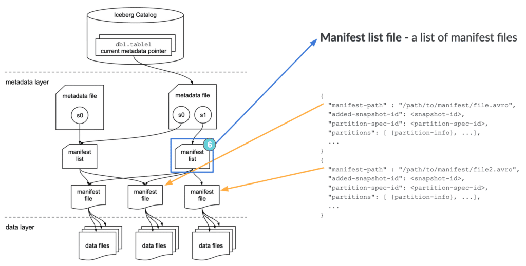
Another aptly named file, the manifest list is a list of manifest files. The manifest list has information about each manifest file that makes up that snapshot, such as the location of the manifest file, what snapshot it was added as part of, and information about the partitions it belongs to and the lower and upper bounds for partition columns for the data files it tracks.
Here’s an example of the full contents of a manifest list file:snap-1257424822184505371-1-eab8490b-8d16-4eb1-ba9e-0dede788ff08.avro (converted to JSON)
{
    "manifest_path": "/home/hadoop/warehouse/db2/part_table2/metadata/eab8490b-8d16-4eb1-ba9e-0dede788ff08-m0.avro",
    "manifest_length": 4884,
    "partition_spec_id": 0,
    "added_snapshot_id": {
        "long": 1257424822184505300
    },
    "added_data_files_count": {
        "int": 1
    },
    "existing_data_files_count": {
        "int": 0
    },
    "deleted_data_files_count": {
        "int": 0
    },
    "partitions": {
        "array": [ {
            "contains_null": false,
            "lower_bound": {
                "bytes": "¹Ô\\u0006\\u0000"
            },
            "upper_bound": {
                "bytes": "¹Ô\\u0006\\u0000"
            }
        } ]
    },
    "added_rows_count": {
        "long": 1
    },
    "existing_rows_count": {
        "long": 0
    },
    "deleted_rows_count": {
        "long": 0
    }
}
{
    "manifest_path": "/home/hadoop/warehouse/db2/part_table2/metadata/d8a778f9-ad19-4e9c-88ff-28f49ec939fa-m0.avro",
    "manifest_length": 4884,
    "partition_spec_id": 0,
    "added_snapshot_id": {
        "long": 8271497753230544000
    },
    "added_data_files_count": {
        "int": 1
    },
    "existing_data_files_count": {
        "int": 0
    },
    "deleted_data_files_count": {
        "int": 0
    },
    "partitions": {
        "array": [ {
            "contains_null": false,
            "lower_bound": {
                "bytes": "¸Ô\\u0006\\u0000"
            },
            "upper_bound": {
                "bytes": "¸Ô\\u0006\\u0000"
            }
        } ]
    },
    "added_rows_count": {
        "long": 1
    },
    "existing_rows_count": {
        "long": 0
    },
    "deleted_rows_count": {
        "long": 0
    }
}
When a SELECT query is reading an Iceberg table and has the manifest list open for the snapshot after getting its location from the metadata file, the query engine then reads the value of the manifest-path entries, and opens the manifest files. It could also do some optimizations at this stage like using row counts or filtering of data using the partition information.
Manifest file
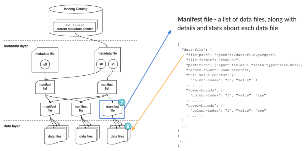
Manifest files track data files as well as additional details and statistics about each file. As mentioned earlier, the primary difference that allows Iceberg to address the problems of the Hive table format is tracking data at the file level — manifest files are the boots on the ground that do that.
Each manifest file keeps track of a subset of the data files for parallelism and reuse efficiency at scale. They contain a lot of useful information that is used to improve efficiency and performance while reading the data from these data files, such as details about partition membership, record count, and lower and upper bounds of columns. These statistics are written for each manifest’s subset of data files during write operation, and are therefore more likely to exist, be accurate, and be up to date than statistics in Hive.
As to not throw the baby out with the bathwater, Iceberg is file-format agnostic, so the manifest files also specify the file format of the data file, such as Parquet, ORC, or Avro.
Here’s an example of the full contents of a manifest file:eab8490b-8d16-4eb1-ba9e-0dede788ff08-m0.avro (converted to JSON)
{
    "status": 1,
    "snapshot_id": {
        "long": 1257424822184505300
    },
    "data_file": {
        "file_path": "/home/hadoop/warehouse/db2/part_table2/data/ts_hour=2021-01-26-01/00000-6-7c6cf3c0-8090-4f15-a4cc-3a3a562eed7b-00001.parquet",
        "file_format": "PARQUET",
        "partition": {
            "ts_hour": {
                "int": 447673
            }
        },
        "record_count": 1,
        "file_size_in_bytes": 973,
        "block_size_in_bytes": 67108864,
        "column_sizes": {
            "array": [ {
                "key": 1,
                "value": 47
            },
            {
                "key": 2,
                "value": 57
            },
            {
                "key": 3,
                "value": 60
            } ]
        },
        "value_counts": {
            "array": [ {
                "key": 1,
                "value": 1
            },
            {
                "key": 2,
                "value": 1
            },
            {
                "key": 3,
                "value": 1
            } ]
        },
        "null_value_counts": {
            "array": [ {
                "key": 1,
                "value": 0
            },
            {
                "key": 2,
                "value": 0
            },
            {
                "key": 3,
                "value": 0
            } ]
        },
        "lower_bounds": {
            "array": [ {
                "key": 1,
                "value": "\\u0002\\u0000\\u0000\\u0000"
            },
            {
                "key": 2,
                "value": "\\u0000„ ,ù\\u0005\\u0000"
            },
            {
                "key": 3,
                "value": "test message 2"
            } ]
        },
        "upper_bounds": {
            "array": [ {
                "key": 1,
                "value": "\\u0002\\u0000\\u0000\\u0000"
            },
            {
                "key": 2,
                "value": "\\u0000„ ,ù\\u0005\\u0000"
            },
            {
                "key": 3,
                "value": "test message 2"
            } ]
        },
        "key_metadata": null,
        "split_offsets": {
            "array": [
                4
            ]
        }
    }
}
When a SELECT query is reading an Iceberg table and has a manifest file open after getting its location from the manifest list, the query engine then reads the value of the file-path entries for each data-file object, and opens the data files. It could also do some optimizations at this stage like using row counts or filtering of data using the partition or column statistic information.
With this understanding of the different components of an Iceberg table and the path taken by any engine or tool accessing data in an Iceberg table, let’s now take a deeper look at what happens under the covers when CRUD operations are performed on an Iceberg table.
A Look Under the Covers When CRUDing
CREATE TABLE
First, let’s create a table in our environment.
CREATE TABLE table1 (
    order_id BIGINT,
    customer_id BIGINT,
    order_amount DECIMAL(10, 2),
    order_ts TIMESTAMP
)
USING iceberg
PARTITIONED BY ( HOUR(order_ts) );
After this statement is executed, the environment will look like this:
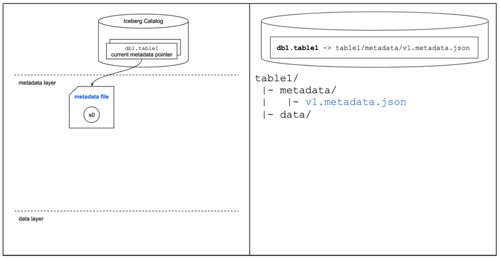
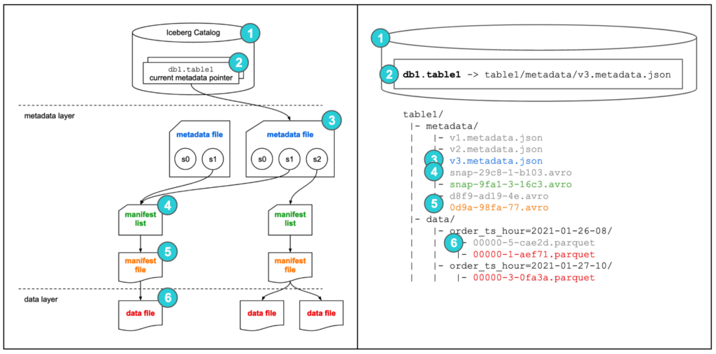
Above, we created a table called table1 in database db1. The table has 4 columns and is partitioned at the hour granularity of the order_ts timestamp column (more on that later).
When the query above is executed, a metadata file with a snapshot s0 is created in the metadata layer (snapshot s0 doesn’t point to any manifest lists because no data exists in the table yet). The catalog entry for db1.table1’s current metadata pointer is then updated to point to the path of this new metadata file.
INSERT
Now, let’s add some data to the table (albeit, literal values).
INSERT INTO table1 VALUES (
    123,
    456,
    36.17,
    '2021-01-26 08:10:23'
);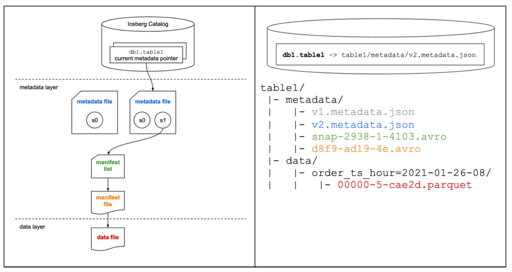
When we execute this INSERT statement, the following process happens:
- The data in the form of a Parquet file is first created –
table1/data/order_ts_hour=2021-01-26-08/00000-5-cae2d.parquet - Then, a manifest file pointing to this data file is created (including the additional details and statistics) –
table1/metadata/d8f9-ad19-4e.avro - Then, a manifest list pointing to this manifest file is created (including the additional details and statistics) –
table1/metadata/snap-2938-1-4103.avro - Then, a new metadata file is created based on the previously current metadata file with a new snapshot
s1as well as keeping track of the previous snapshots0, pointing to this manifest list (including the additional details and statistics) –table1/metadata/v2.metadata.json - Then, the value of the current metadata pointer for
db1.table1is atomically updated in the catalog to now point to this new metadata file.
During all of these steps, anyone reading the table would continue to read the first metadata file until the atomic step #5 is complete, meaning that no one using the data would ever see an inconsistent view of the table’s state and contents.
MERGE INTO / UPSERT
Now, let’s step through a MERGE INTO / UPSERT operation.
Let’s assume we’ve landed some data into a staging table we created in the background. In this simple example, information is logged each time there’s a change to the order, and we want to keep this table showing the most recent details of each order, so we update the order amount if the order ID is already in the table. If we don’t have a record of that order yet, we want to insert a record for this new order.
In this example, the stage table includes an update for the order that’s already in the table (order_id=123) and a new order that isn’t in the table yet, which occurred on January 27, 2021 at 10:21:46.
MERGE INTO table1
USING ( SELECT * FROM table1_stage ) s
    ON table1.order_id = s.order_id
WHEN MATCHED THEN
    UPDATE table1.order_amount = s.order_amount
WHEN NOT MATCHED THEN
    INSERT *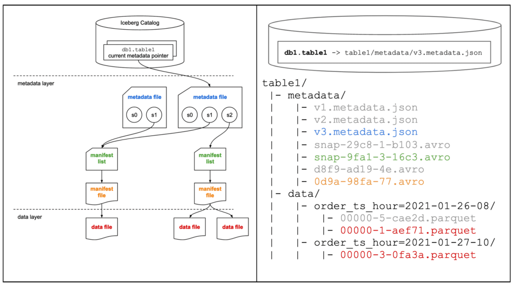
When we execute this MERGE INTO statement, the following process happens:
- The read path as detailed earlier is followed to determine all records in
table1andtable1_stagethat have the sameorder_id. - The file containing the record with
order_id=123fromtable1is read into the query engine’s memory (00000-5-cae2d.parquet),order_id=123’s record in this memory copy then has itsorder_amountfield updated to reflect the neworder_amountof the matching record intable1_stage. This modified copy of the original file is then written to a new Parquet file –table1/data/order_ts_hour=2021-01-26-08/00000-1-aef71.parquet- Even if there were other records in the file that didn’t match the
order_idupdate condition, the entire file would still be copied and the one matching record updated as it was copied, and the new file written out — a strategy known as copy-on-write. There is a new data change strategy coming soon in Iceberg known as merge-on-read which will behave differently under the covers, but still provides you the same update and delete functionality.
- Even if there were other records in the file that didn’t match the
- The record in
table1_stagethat didn’t match any records intable1gets written in the form of a new Parquet file, because it belongs to a different partition than the matching record –table1/data/order_ts_hour=2021-01-27-10/00000-3-0fa3a.parquet - Then, a new manifest file pointing to these two data files is created (including the additional details and statistics) –
table1/metadata/0d9a-98fa-77.avro- In this case, the only record in the only data file in snapshot
s1was changed, so there was no reuse of manifest files or data files. Normally this is not the case, and manifest files and data files are reused across snapshots.
- In this case, the only record in the only data file in snapshot
- Then, a new manifest list pointing to this manifest file is created (including the additional details and statistics) –
table1/metadata/snap-9fa1-3-16c3.avro - Then, a new metadata file is created based on the previously current metadata file with a new snapshot
s2as well as keeping track of the previous snapshotss0ands1, pointing to this manifest list (including the additional details and statistics) –table1/metadata/v3.metadata.json - Then, the value of the current metadata pointer for
db1.table1is atomically updated in the catalog to now point to this new metadata file.
While there are multiple steps to this process, it all happens quickly. One example is where Adobe did some benchmarking and found they could achieve 15 commits per minute.
In the diagram above, we also show that before this MERGE INTO was executed, a background garbage collection job ran to clean up unused metadata files — note that our first metadata file for snapshot s0 when we created the table is no longer there. Because each new metadata file also contains the important information needed from previous ones, these can be cleaned up safely. Unused manifest lists, manifest files, and data files can also be cleaned up via garbage collection.
SELECT
Let’s review the SELECT path again, but this time on the Iceberg table we’ve been working on.
SELECT *
FROM db1.table1
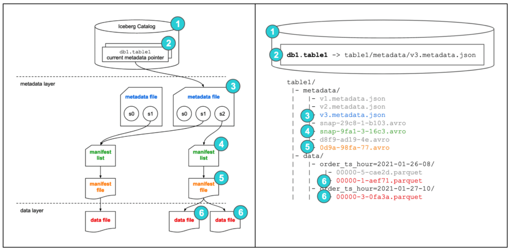
When this SELECT statement is executed, the following process happens:
- The query engine goes to the Iceberg catalog
- It then retrieves the current metadata file location entry for
db1.table1 - It then opens this metadata file and retrieves the entry for the manifest list location for the current snapshot,
s2 - It then opens this manifest list, retrieving the location of the only manifest file
- It then opens this manifest file, retrieving the location of the two data files
- It then reads these data files, and since it’s a
SELECT *, returns the data back to the client
Hidden Partitioning
Recall earlier in this post we discussed one of the problems of the Hive table format is that the users need to know the physical layout of the table in order to avoid very slow queries.
Let’s say a user wants to see all records for a single day, say January 26, 2021, so they issue this query:
SELECT *
FROM table1
WHERE order_ts = DATE '2021-01-26'
Recall that when we created the table, we partitioned it at the hour-level of the timestamp of when the order first occurred. In Hive, this query generally causes a full table scan.
Let’s walk through how Iceberg addresses this problem and provides users with the ability to interact with the table in an intuitive way while still achieving good performance, avoiding a full table scan.
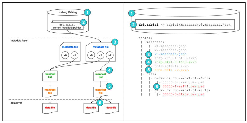
When this SELECT statement is executed, the following process happens:
- The query engine goes to the Iceberg catalog.
- It then retrieves the current metadata file location entry for
db1.table1. - It then opens this metadata file, retrieves the entry for the manifest list location for the current snapshot
s2. It also looks up the partition specification in the file and sees that the table is partitioned at the hour level of theorder_tsfield. - It then opens this manifest list, retrieving the location of the only manifest file.
- It then opens this manifest file, looking at each data file’s entry to compare the partition value the data file belongs to with the one requested by the user’s query. The value in this file corresponds to the number of hours since the Unix epoch, which the engine then uses to determine that only the events in one of the data files occurred on January 26, 2021 (or in other words, between January 26, 2021 at 00:00:00 and January 26, 2021 at 23:59:59).
- Specifically, the only event that matched is the first event we inserted, since it happened on January 26, 2021 at 08:10:23. The other data file’s order timestamp was January 27, 2021 at 10:21:46, i.e., not on January 26, 2021, so it didn’t match the filter.
- It then only reads the one matching data file, and since it’s a
SELECT *, it returns the data back to the client.
Time Travel
Another key capability the Iceberg table format enables is something called “time travel.”
To keep track of the state of a table over time for compliance, reporting, or reproducibility purposes, data engineering traditionally needs to write and manage jobs that create and manage copies of the table at certain points in time.
Instead, Iceberg provides the ability out-of-the-box to see what a table looked like at different points in time in the past.
For instance, let’s say that today a user needed to see the contents of our table as of January 28, 2021, and since this is a static text article, let’s say was before the order from January 27 was inserted into the table and before the order from January 26 had its order amount updated via the UPSERT operation we did above. Their query would look like this:
SELECT *
FROM table1 AS OF '2021-01-28 00:00:00'
-- (timestamp is from before UPSERT operation)
When this SELECT statement is executed, the following process happens:
- The query engine goes to the Iceberg catalog
- It then retrieves the current metadata file location entry for
db1.table1 - It then opens this metadata file and looks at the entries in the
snapshotsarray (which contains the millisecond Unix epoch time the snapshot was created, and therefore became the most current snapshot), determines which snapshot was active as of the requested point in time (January 28, 2021 at midnight), and retrieves the entry for the manifest list location for that snapshot, which iss1 - It then opens this manifest list, retrieving the location of the only manifest file
- It then opens this manifest file, retrieving the location of the two data files
- It then reads these data files, and since it’s a
SELECT *, returns the data back to the client
Notice in the file structure in the diagram above, that although the old manifest list, manifest file, and data files are not used in the current state of the table, they still exist in the data lake and are available for use.
Of course, while keeping around old metadata and data files provides value in these use cases, at a certain point you’ll have metadata and data files that are either no longer accessed or the value of allowing people to access them outweighs the cost of keeping them. So, there is an asynchronous background process that cleans up old files called garbage collection. Garbage collection policies can be configured according to the business requirements, and is a trade-off between how much storage you want to use for old files versus how far back in time and at what granularity you want to provide.
Compaction
Another key capability available as part of Iceberg’s design is compaction, which helps balance the write-side and read-side trade-offs.
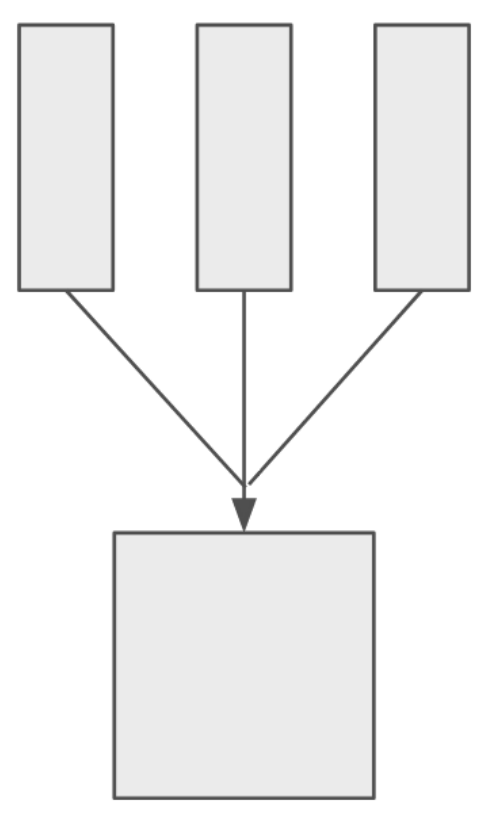
In Iceberg, compaction is an asynchronous background process that compacts a set of small files into fewer larger files. Since it’s asynchronous and in the background, it has no negative impact on your users. In fact, it’s basically a specific kind of a normal Iceberg write job that has the same records as input and output, but the file sizes and attributes are far improved for analytics after the write job commits its transaction.
Anytime you’re working with data, there are trade-offs for what you’re looking to achieve, and in general the incentives on the write-side and read-side pull in opposite directions.
- On the write-side, you generally want low latency — making the data available as soon as possible, meaning you want to write as soon as you get the record, potentially without even converting it into a columnar format. But, if you were to do this for every record, you would end up with one record per file (the most extreme form of the small files problem).
- On the read-side, you generally want high throughput — having many many records in a single file and in a columnar format, so your data-correlated variable costs (reading the data) outweigh your fixed costs (overhead of record-keeping, opening each file, etc.). You also generally want up-to-date data, but you pay the cost of that on read operations.
Compaction helps balance the write-side and read-side trade-offs — you can write the data close to as soon as you get it, which at the extreme would be 1 record in row format per file which readers can see and use right away, while a background compaction process periodically takes all those small files and combines them into fewer, larger, columnar format files.
With compaction, your readers continually have 99% of their data in the high-throughput form they want, but still see the most recent 1% of data in the low-latency low-throughput form.
It’s also important to note for this use case that the input file format and output file format of compaction jobs can be different file types. A good example of this would be writing Avro from streaming writes, which are compacted into larger Parquet files for analytics.
Another important note, since Iceberg is not an engine or tool, scheduling/triggering and the actual compaction work is done by other tools and engines that integrate with Iceberg.
Design Benefits of the Format
Now, let’s apply what we’ve gone through so far to the higher-level value the architecture and design provides.
- Snapshot isolation for transactions
- Reads and writes on Iceberg tables don’t interfere with each other.
- Iceberg provides the ability for concurrent writes via Optimistic Concurrency Control.
- All writes are atomic.
- Faster planning and execution
- Both of these benefits stem from the fact that you’re writing details about what you’ve written on the write-path, versus getting that information on the read-path.
- Because the list of files are written when changes to the table are made, there’s no need to do expensive filesystem list operations at runtime, meaning there is far less work and waiting to do at runtime.
- Because statistics about the data in the files is written on the write-side, statistics aren’t missing, wrong, or out of date, meaning cost-based optimizers can make better decisions in deciding which query plan provides the fastest response time.
- Because statistics about the data in the files is tracked at the file level, the statistics aren’t as coarse-grained, meaning engines can do more data pruning, process less data, and therefore have faster response times.
- In Ryan Blue’s presentation linked earlier in this article, he shares the results of an example use case at Netflix:
- For a query on a Hive table, it took 9.6 minutes just to plan the query
- For the same query on an Iceberg table, it only took 42 seconds to plan and execute the query
- Abstract the physical, expose a logical view
- Earlier in this article, we saw that with Hive tables, users often need to know the potentially unintuitive physical layout of the table in order to achieve even decent performance.
- Iceberg provides the ability to continually expose a logical view to your users, decoupling the logical interaction point from the physical layout of the data. We saw how this is incredibly useful with capabilities like hidden partitioning and compaction.
- Iceberg provides the ability to transparently evolve your table over time, via schema evolution, partition evolution, and sort order evolution capabilities. More details on these can be found on the Iceberg docs site.
- It is much easier for data engineering to experiment with different, potentially better, table layouts behind the scenes. Once committed, the changes will take effect without users having to change their application code or queries. If an experiment turns out to make things worse, the transaction can be rolled back and users are returned to the previous experience. Making experimentation safer allows more experiments to be performed and therefore allows you to find out better ways of doing things.
- All engines see changes immediately
- Because the files making up a table’s contents are defined on the write-side, and as soon as the file list changes all new readers are pointed to this new list (via the read flow starting at the catalog), as soon as a writer makes a change to the table, all new queries using this table immediately see the new data.
- Event listeners
- Iceberg has a framework that allows other services to be notified when an event occurs on an Iceberg table. Currently, this feature is in the early stages, and only an event when a table is scanned can be emitted. This framework, however, provides the ability for future capabilities, such as keeping caches, materialized views, and indexes in sync with the raw data.
- Efficiently make smaller updates
- Because data is tracked at the file level, smaller updates can be made to the dataset much more efficiently.
Try Dremio’s Interactive Demo
Explore this interactive demo and see how Dremio's Intelligent Lakehouse enables Agentic AI
