This article has been revised and updated from its original version published in 2022 to reflect the latest Apache Iceberg developments, including V3 deletion vectors.
Apache Iceberg supports row-level operations (UPDATE, DELETE, and MERGE) through two fundamentally different strategies: Copy-on-Write (COW) and Merge-on-Read (MOR). Each strategy makes different tradeoffs between write performance and read performance, and choosing the right one for your workload can mean the difference between a pipeline that takes seconds and one that takes hours.
V3 of the Iceberg specification introduces a third option (deletion vectors) that combines the best characteristics of both approaches. This guide explains how each strategy works, when to use it, and how V3 deletion vectors change the calculus.
Why Row-Level Changes Are Hard on Object Storage
Object storage (S3, GCS, ADLS) is immutable, you can't modify a file in place. To change a single row in a 256MB Parquet file, you have fundamentally two choices: For official documentation, refer to the Iceberg delete format specification.
Rewrite the entire file without the old row and with the new row (Copy-on-Write)
Write a small "delete marker" file that tells readers to skip the old row, and write a new file with the updated row (Merge-on-Read)
Traditional databases can update rows in place because their storage format supports random writes. Object storage doesn't, so Iceberg must choose one of these two strategies, each with significant tradeoffs.
Try Dremio’s Interactive Demo
Explore this interactive demo and see how Dremio's Intelligent Lakehouse enables Agentic AI
Copy-on-Write (COW): How It Works
When you execute a DELETE, UPDATE, or MERGE with Copy-on-Write mode:
Identify affected files: The engine reads manifest entries to find which data files contain rows matching the condition (using column statistics pruning)
Read affected files entirely: Every affected data file is downloaded and deserialized, even if only one row in that file matches the condition
Apply changes in memory: Delete matching rows, apply updates, or merge new data
Write new files: Serialize the modified data into new Parquet files and upload them to object storage
Commit: Create a new snapshot where the manifest points to the new files instead of the old ones
COW Example: Deleting a Customer's Data
DELETE FROM orders WHERE customer_id = 42;
If customer 42's orders are spread across 50 data files (256MB each), COW must:
Download all 50 files (12.5GB total)
Remove customer 42's rows (maybe 100 rows out of millions)
Write 50 new files (nearly identical to the originals)
Upload 12.5GB back to storage
The old files remain on storage until snapshot expiry and orphan cleanup remove them.
COW Performance Characteristics
Metric
Impact
Write cost
High, rewrites entire affected files
Read cost
Zero overhead, data files are always clean
Write amplification
Very high, changing 1 row rewrites entire file
Storage overhead
Temporary 2x (old + new files until expiry)
Best for
Read-heavy workloads with infrequent updates
Merge-on-Read (MOR): How It Works
Merge-on-Read avoids rewriting data files entirely. Instead, it records which rows should be considered deleted:
Identify affected rows: Find which rows in which files match the condition
Write delete files: Create small Avro or Parquet files that record the deleted row positions or equality conditions
Write new data files (for UPDATE/MERGE), Write only the new/updated rows
Commit: Create a new snapshot that includes both the original data files AND the new delete files
Delete File Types (V2)
Iceberg V2 supports two types of delete files:
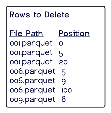
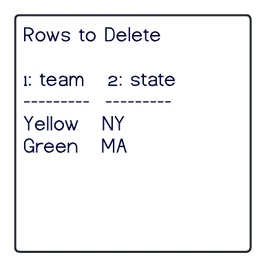
Positional Delete Files: Record the file path and row position of each deleted row:
Equality Delete Files: Record column values that identify deleted rows:
customer_id
42
Any row in any data file where customer_id = 42 is treated as deleted. More flexible but more expensive to evaluate at read time.
MOR Read-Time Merge
When a query reads a MOR table, the engine must merge data files with delete files:
Read the data file
Read all associated delete files
For each row in the data, check if it appears in any delete file
Skip matched rows in the query results
This merge adds overhead to every read operation. The overhead grows as delete files accumulate.
MOR Example: Same Delete as Above
DELETE FROM orders WHERE customer_id = 42;
With MOR:
Write one small equality delete file: {customer_id: 42} (a few bytes)
No data files are rewritten
Commit takes milliseconds
The write is dramatically faster, but every subsequent query on this table must check the delete file during reads.
MOR Performance Characteristics
Metric
Impact
Write cost
Very low, only writes small delete files
Read cost
Moderate to high, must merge delete files with data files
Write amplification
Minimal, no data rewriting
Storage overhead
Low, only small delete files added
Best for
Write-heavy workloads, streaming, CDC ingestion
V3 Deletion Vectors: The Best of Both
Iceberg V3 introduces deletion vectors, a bitmap-based approach that combines fast writes with fast reads:
How Deletion Vectors Work
Instead of writing separate delete files, V3 stores a compact bitmap alongside each data file's manifest entry. The bitmap marks which row positions are deleted:
Data File: s3://warehouse/data/00042.parquet (125,000 rows)
Deletion Vector: bitmap [0,0,0...,1...,0,1...,0]  (rows 1547 and 8923 deleted)
Why This Is Faster
Operation
V2 MOR
V3 Deletion Vectors
Write a delete
Write a new Avro delete file
Set bits in bitmap (metadata-only)
Read with deletes
Download and join delete file
Check bitmap (in-memory, O(1) per row)
Accumulation
Many delete files degrade reads
Bitmaps merge efficiently
Deletion vectors eliminate the separate delete file entirely. The reader checks a compact bitmap during the scan (an O(1) operation per row) instead of joining against a potentially large delete file.
When to Use Deletion Vectors
V3 deletion vectors are the recommended approach for most workloads going forward. They supersede the V2 MOR approach for:
Set the strategy per operation type using table properties:
-- Set delete mode
ALTER TABLE orders SET TBLPROPERTIES (
  'write.delete.mode' = 'merge-on-read'
);

-- Set update mode
ALTER TABLE orders SET TBLPROPERTIES (
  'write.update.mode' = 'merge-on-read'
);

-- Set merge mode
ALTER TABLE orders SET TBLPROPERTIES (
  'write.merge.mode' = 'merge-on-read'
);
You can mix strategies, for example, use COW for updates (to keep clean files) but MOR for deletes (since deletes are typically less frequent and affect fewer files).
Compaction: Resolving MOR Overhead
The key insight about MOR is that it's a deferred strategy, it trades immediate write cost for ongoing read cost. Compaction is how you resolve that deferred cost:
Run MOR writes throughout the day (fast writes, accumulating delete files)
Run compaction during a maintenance window
Compaction reads data files + delete files → writes new, clean data files
After compaction, reads are as fast as COW
This pattern gives you the best of both worlds: fast writes during production hours and fast reads after compaction. Dremio automates this lifecycle for managed tables.
Engine Support
Engine
COW
MOR (V2)
Deletion Vectors (V3)
Apache Spark
Full
Full
Full (3.5+)
Dremio
Full
Full
Full
Apache Flink
Full
Full
Partial
Trino
Full
Full
In progress
StarRocks
Full
Full
Full
Impact on Related Features
The write mode affects several other Iceberg features:
Time travel: Both COW and MOR snapshots are valid for time travel. MOR snapshots include delete files.
Rollback: Rolling back a MOR commit removes the delete files, restoring the original data.
Performance tuning: MOR with many delete files reduces pruning effectiveness. Sort order and compaction mitigate this.
GDPR compliance: MOR provides fast initial compliance (data is logically deleted). Compaction + snapshot expiry provides full data erasure.
Real-World Performance Comparison
Understanding the concrete impact helps you make the right choice. Here are typical numbers for a 1TB orders table with 3,000 data files:
These numbers make the case clearly: COW is only appropriate when updates are infrequent and reads are the dominant workload. For any workload with regular row-level changes, MOR or deletion vectors are far more efficient.
Migrating Between Strategies
Changing your write mode doesn't require rewriting existing data. The change takes effect for new writes only:
-- Switch from COW to MOR
ALTER TABLE orders SET TBLPROPERTIES (
  'write.delete.mode' = 'merge-on-read',
  'write.update.mode' = 'merge-on-read',
  'write.merge.mode' = 'merge-on-read'
);
After switching:
Existing data files remain unchanged (they were written by COW, so they're clean)
New row-level operations create delete files (MOR)
Queries handle both smoothly, the engine knows which files have associated delete files
To upgrade to V3 deletion vectors, you must also upgrade the table's format version:
ALTER TABLE orders SET TBLPROPERTIES (
  'format-version' = '3'
);
This is a metadata-only change. No data files are rewritten. However, you should verify that all engines reading this table support V3 before upgrading.
Common Questions
Can I use different strategies for different operations on the same table?
Yes. You can set write.delete.mode, write.update.mode, and write.merge.mode independently. A common pattern is COW for updates (to keep frequently queried columns clean) and MOR for deletes (since deletes are typically less frequent).
How many delete files is too many?
It depends on your query latency requirements. As a rule of thumb, if your query planning starts showing significant time spent on "merge delete files" in the query profile, it's time to run compaction. For most workloads, compacting when more than 50-100 delete files accumulate per partition is a good threshold.
Do Dremio Reflections work with MOR tables?
Yes. Dremio's Reflections are themselves Iceberg tables managed by Dremio. When the source table has new MOR writes, Reflections are incrementally updated. Queries hitting Reflections always see clean, optimally sorted data regardless of the source table's write mode.
Is V3 backward compatible?
V3 tables can be read by engines that support V3. Engines that only support V2 cannot read V3 deletion vectors. Before upgrading, ensure all consumers of the table support V3. The major engines (Spark 3.5+, Dremio, StarRocks) all support V3.
Frequently Asked Questions
When should I use copy-on-write vs merge-on-read?
Use copy-on-write when your workload has infrequent updates and high read frequency, since it optimizes for read performance at the cost of write latency. Use merge-on-read when you have frequent updates (CDC pipelines, streaming upserts) and can tolerate slightly higher read overhead. V3 deletion vectors significantly reduce the read overhead of merge-on-read, making it the preferred default for most workloads.
Can I switch between COW and MOR on the same table?
Yes. The write mode is a table property that you can change at any time. Existing data files remain in their original format, and new writes use the updated strategy. This lets you adjust based on evolving workload patterns without migrating data.
How do delete files affect query performance over time?
Delete files accumulate with each merge-on-read delete or update operation. As the number of delete files grows, each read must merge them with the data files, increasing query latency. Regular compaction resolves this by rewriting data files with deletes applied, returning read performance to baseline levels.
The ability to update and delete rows in traditional databases is something that was always needed, and was always available, yet we took for granted. Data warehouses, which are essentially specialized databases for analytics, have been around a long time and evolved from those very features. They are easier to implement as they internally handle the storage and processing of data.
Data lakes exist to solve cost and scale challenges, and is achieved by using independent technologies to solve problems like storage, compute and more. Storage at scale was solved by the advent of cloud object storage, and compute engines evolved to handle read-only queries at scale. In today’s world, the idea of the data lakehouse promises cost savings and scalability in moving traditionally data warehouse workloads to the data lake.
To facilitate these kinds of workloads, which include many write-intensive workloads, data lakes needed new abstractions between storage and compute to help provide ACID guarantees and performance. And this is what data lake table formats provide: a layer of abstraction for data lakehouse engines to look at your data as well-defined tables that can be operated on at scale.
Apache Iceberg is a table format that serves as the layer between storage and compute to provide analytics at scale on the lake, manifesting the promise of the data lakehouse.
While Apache Iceberg delivers ACID guarantees with updates/deletes to the data lakehouse, version 2 (v2) of the Apache Iceberg table format offers the ability to update and delete rows to enable more use cases. V2 of the format enables updating and deleting individual rows in immutable data files without rewriting the files.
There are two approaches to handle deletes and updates in the data lakehouse: copy-on-write (COW) and merge-on-read (MOR).
Like with almost everything in computing, there isn’t a one-size-fits-all approach – each strategy has trade-offs that make it the better choice in certain situations. The considerations largely come down to latency on the read versus write side. These considerations aren't unique to Iceberg or data lakes in general, the same considerations and trade-offs exist in many other places, such as lambda architecture.
The following walks through how each of the strategies work, identifies their pros and cons, and discusses which situations are best for their use.
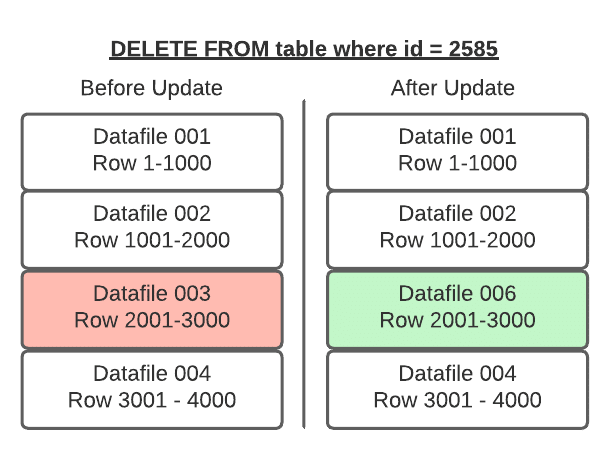
Copy-On-Write (COW) – Best for tables with frequent reads, infrequent writes/updates, or large batch updates
With COW, when a change is made to delete or update a particular row or rows, the datafiles with those rows are duplicated, but the new version has the updated rows. This makes writes slower depending on how many data files must be re-written which can lead to concurrent writes having conflicts and potentially exceeding the number of reattempts and failing.
If updating a large number of rows, COW is ideal. However, if updating just a few rows you still have to rewrite the entire data file, making small or frequent changes expensive.
On the read side, COW is ideal as there is no additional data processing needed for reads – the read query has nice big files to read with high throughput.
Summary of COW (Copy-On-Write)
PROS
CONS
Fastest reads
Expensive writes
Good for infrequent updates/deletes
Bad for frequent updates/deletes
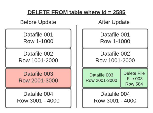
Merge-On-Read (MOR) – Best for tables with frequent writes/updates
With merge-on-read, the file is not rewritten, instead the changes are written to a new file. Then when the data is read, the changes are applied or merged to the original data file to form the new state of the data during processing.
This makes writing the changes much quicker, but also means more work must be done when the data is read.
In Apache Iceberg tables, this pattern is implemented through the use of delete files that track updates to existing data files.
If you delete a row, it gets added to a delete file and reconciled on each subsequent read till the files undergo compaction which will rewrite all the data into new files that won’t require the need for the delete file.
If you update a row, that row is tracked via a delete file so future reads ignore it from the old data file and the updated row is added to a new data file. Again, once compaction is run, all the data will be in fewer data files and the delete files will no longer be needed.
So when a query is underway the changes listed in the delete files will be applied to the appropriate data files before executing the query.
Position Deletes
Position deletes still read files to determine which records are deleted, but instead of rewriting the data files after the read, it only writes a delete file that tracks the file and position in that file of records to be deleted. This strategy greatly reduces write times for updates and deletes, and there is a minor cost to merge the delete files at read time.
Equality Deletes
When using equality deletes, you save even more time during the write by avoiding reading any files at all. Instead, the delete file is written to include the fields and values that are targeted by the query. This makes update/delete writes much faster than using position deletes. However, there is a much higher cost on the read time since it will have to match the delete criteria against all scanned rows to reconcile at read, which can be quite costly.
Minimizing the Read Costs
When running compaction, new data files will be written to reconcile any existing delete files, eliminating the need to reconcile them during read queries. So when using merge-on-read, it is recommended to have regular compaction jobs to impact reads as little as possible while still maintaining the faster write speeds.
Types of Delete Files Summary
How it works
Pros
Cons
How to manage read costs
Good fit
Position
Tracks file path and row position in file
Fast writes
Slower reads
Run compaction jobs regularly
Better for frequent updates/deletes in which copy- on-write is not fast enough
Equality
Tracks query criteria for delete/update targets
Super-fast writes
Much slower reads
For when updates/deletes with position deletes is still not fast enough
How it works
Pros
Cons
How to manage read costs
Good fit
Position
Tracks file path and row position in file
Fast writes
Slower reads
Run compaction jobs regularly
Better for frequent updates/deletes in which copy- on-write is not fast enough
Equality
Tracks query criteria for delete/update targets
Super- fast writes
Much slower reads
For when updates/deletes with position deletes is still not fast enough
When to Use COW and When to Use MOR
Architecting your tables to take advantage of COW, MOR/Position deletes or MOR/Equality deletes is based on how the table will be used.
Note that you can choose a strategy you believe is the best option for your table, and if it turns out to be the wrong choice or the workloads change, it’s easy to change the table to use another.
Approach
Update/Delete Frequency
Insert Performance
Update/Delete Latency/Performance
Read Latency/ Performance
Copy-On-Write
Infrequent updates/deletes
Same
Slowest
Fastest
Merge-On-Read Position Deletes
Frequent updates/deletes
Same
Fast
Fast
Merge-On-Read Equality Deletes
Frequent updates/deletes where position delete MOR is still not fast enough on the write side
Same
Fastest
Slowest
Configuring COW and MOR
COW and MOR are not an either/or proposition with Apache Iceberg. You can specify different modes in your table settings based on the type of operation, so you can specify deletes, updates, and merges as either COW or MOR independently. For example, you can set the settings when the table is created.
CREATE TABLE catalog.db.students (
    id int,
    first_name string,
    last_name string,
    major string,
    class_year int
) TBLPROPERTIES (
    'write.delete.mode'='copy-on-write',
    'write.update.mode'='merge-on-read',
    'write.merge.mode'='merge-on-read'
) PARTITIONED BY (class_year) USING iceberg;
This can also be changed using ALTER TABLE statements:
ALTER TABLE catalog.db.students SET TBLPROPERTIES (
    'write.delete.mode'='merge-on-read',
    'write.update.mode'='copy-on-write',
    'write.merge.mode'='copy-on-write'
);
Further Optional Delete/Updates Fine-Tuning Strategies
Partitioning the table by fields that are often included in query filters, so if you regularly filter a field by a particular timestamp field during updates, then partitioning the table by that field will speed updates.
Sorting the table by fields often included in the filters (Example: if table partitioned by day(timestamp) setting the sort key to timestamp).
Tuning the metadata tracked for each individual column so extra metadata isn’t written for columns the table is rarely filtered by, ultimately wasting time on the write side. This can be done with the write.metadata.metrics category or properties to set a default rule and also customize each column.
ALTER TABLE catalog.db.students SET TBLPROPERTIES (
    'write.metadata.metrics.column.col1'='none',
    'write.metadata.metrics.column.col2'='full',
    'write.metadata.metrics.column.col3'='counts',
    'write.metadata.metrics.column.col4'='truncate(16)',
);
Fine-tuning at the engine level, which will differ based on the engine you are using. For example, for streaming ingestion where you’re confident there won’t be schema fluctuations in the incoming data, you may want to tweak certain Iceberg-specific Spark write settings such as disabling the “check-ordering” setting which would save time by not checking that the data being written has the fields in the same order as the table.
With Apache Iceberg v2 tables, you now have more flexibility to handle deletes, updates, and upserts so you can choose the trade-offs between writes and reads to engineer the best performance for your particular workloads. Using copy-on-write, merge-on-read, position deletes, and equality deletes gives you the flexibility to tailor how engines update in your Iceberg tables.
Try Dremio Cloud free for 30 days
Deploy agentic analytics directly on Apache Iceberg data with no pipelines and no added overhead.
Ingesting Data Into Apache Iceberg Tables with Dremio: A Unified Path to Iceberg
By unifying data from diverse sources, simplifying data operations, and providing powerful tools for data management, Dremio stands out as a comprehensive solution for modern data needs. Whether you are a data engineer, business analyst, or data scientist, harnessing the combined power of Dremio and Apache Iceberg will undoubtedly be a valuable asset in your data management toolkit.
Sep 22, 2023·Dremio Blog: Open Data Insights
Intro to Dremio, Nessie, and Apache Iceberg on Your Laptop
We're always looking for ways to better handle and save money on our data. That's why the "data lakehouse" is becoming so popular. It offers a mix of the flexibility of data lakes and the ease of use and performance of data warehouses. The goal? Make data handling easier and cheaper. So, how do we […]
Oct 12, 2023·Product Insights from the Dremio Blog
Table-Driven Access Policies Using Subqueries
This blog helps you learn about table-driven access policies in Dremio Cloud and Dremio Software v24.1+.