Accelerating Joins in Dremio with Runtime Filters

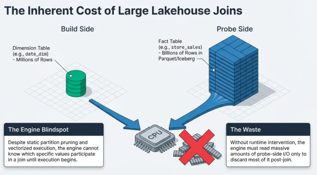
Modern lakehouse workloads are full of large joins. A typical BI query might join a few million rows of dimension data to billions of rows in a fact table stored as Parquet or Iceberg. Even when the result set is small, the engine often has to read and process a huge amount of data on the "big" side of the join before it can throw most of it away.

In Dremio, the engine already leans on partition pruning, file pruning, reflections, and vectorized execution to make those joins fast. But there's still a gap: the engine doesn't know which values actually participate in the join until the query is running.

Runtime filters close that gap.

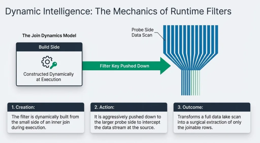
At a high level, runtime filters let Dremio learn from the smaller side of an inner join while the query is executing, build a compact filter from the observed join keys, and push that filter down to the larger side of the join. That filter can then be used to prune partitions and files and even filter rows on the probe side, often turning "scan most of the data lake" into "scan just the data that can possibly join".

In this post, we'll look at how runtime filters work in Dremio, how they interact with the execution timeline and backpressure, and when you can expect them to deliver big performance wins.

Build Side, Probe Side, and the Cost of Big Joins

Before we get into runtime filters, it's worth revisiting how Dremio executes a hash join.

For an inner join, the planner chooses:

• Build side - the smaller input. Dremio reads this input first and builds an in-memory hash table keyed on the join columns.
• Probe side - the larger input. Dremio streams batches from this input and probes the hash table to find matches.

In a star-schema style query, dimension tables like customer, item, or date_dim are good build-side candidates, while large fact tables like store_sales or web_sales are natural probe sides.

The expensive part of the join is usually the probe side scan. If we read a large Iceberg or Parquet-backed fact table and only a small fraction of rows actually join, most of the I/O and CPU spent on the probe side is wasted work.

This is exactly where runtime filters step in.

What Are Runtime Filters in Dremio?

Conceptually, a runtime filter is a filter that is constructed during execution from the build side of an inner join and pushed down to the probe side.

At a high level:

1. The build side of the join runs and populates an in-memory hash table with the join keys it sees.
2. After the build side has finished, Dremio compresses those keys into a compact data structure (for example, a Bloom filter or small value set) that can be shipped across the cluster.
3. Once the runtime filter is ready, Dremio broadcasts it to all the scan fragments that are reading the probe side.
4. Those scans use the runtime filter to prune work on the probe side by:
   • Skipping partitions and, in some cases, entire data files that cannot contain matching keys, based on partition information and file-level metadata (for example, Iceberg manifests).
   • Optionally filtering rows using the runtime filter where appropriate.

The key property is that this filter is generated at runtime - the engine doesn't know its contents at planning time, because it doesn't yet know which keys will appear on the build side for this specific query.

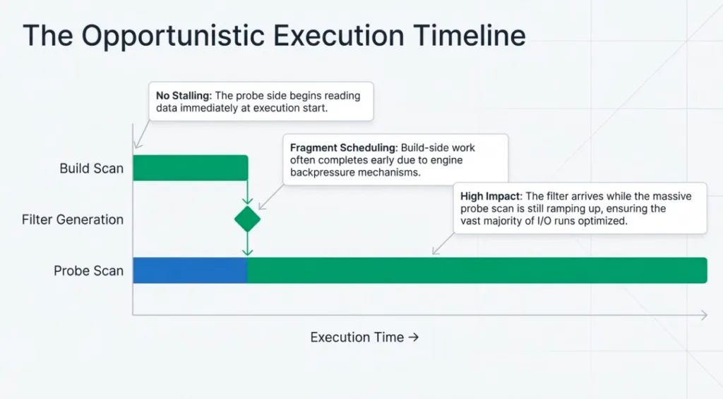
Equally important: Dremio does not stall the entire query waiting for this filter to exist. The probe side still starts reading as usual. The runtime filter is an opportunistic optimization: the later it arrives relative to the total probe scan, the less it can optimize; the earlier it arrives, the more of the probe side it can pruned optimizing the query.

Where Runtime Filters Apply: Partitions, Files, and Row Groups

On Iceberg- and Parquet-backed tables, runtime filters can be applied at several layers in the plan:

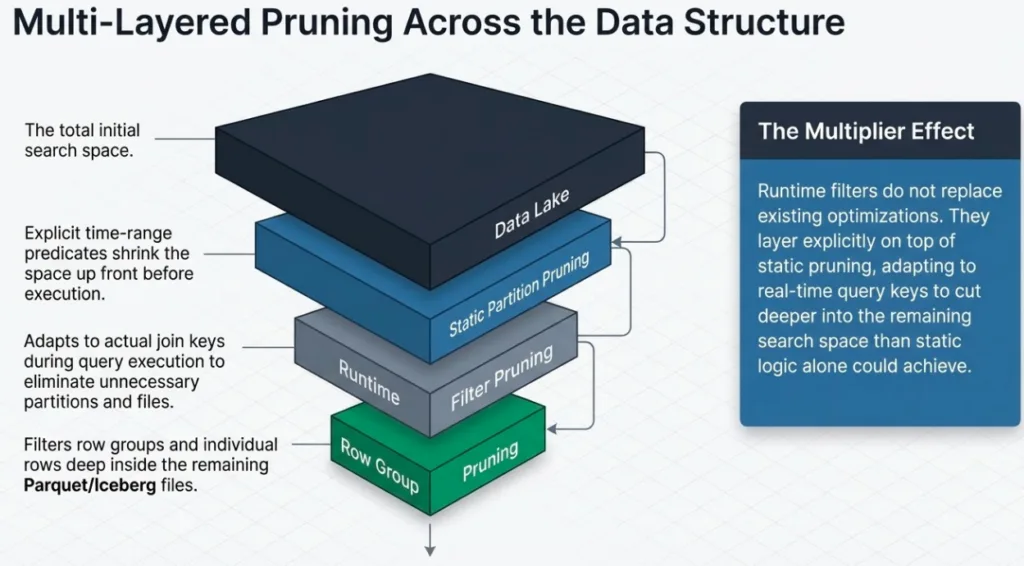
• Partition and file-level pruning
  When the join key (or a strongly correlated key) is part of the partition spec or reflected in file-level metadata, Dremio can use the runtime filter to drop entire partitions or data files on the probe side. For filesystem and Hive sources this typically means skipping partitions or splits based on partition values; for Iceberg tables it also means leveraging manifest and file-level statistics to skip whole data files up front. These files are never scheduled or read, which is usually the biggest I/O and CPU win.
• Row-group-level pruning with metadata and Bloom filters
  Within a Parquet file, Dremio can intersect the runtime filter with row-group metadata (a row group is a horizontal chunk of rows stored together with shared statistics and indexes), including min/max statistics, dictionaries, and Bloom filters, to skip entire row groups that cannot contain matching keys. The file is opened, but large chunks inside it are never read or processed.
• Row-level filtering
  Even when partitioning or row-group metadata do not line up perfectly with the join key, the runtime filter can still act as part of a row-level predicate on the probe side (for example, in Parquet readers). This does not save as much I/O as dropping files or row groups, but it still reduces the amount of data flowing into the join and the number of comparisons the join has to perform. In practice, this row-level behavior is governed by runtime-filter configuration options and format support, so the exact degree of row-level filtering may vary by deployment.

In many real queries you will see a combination of static filters (for example, an explicit time-range predicate on a partition key) and runtime filters on join keys. The static filters shrink the search space up front, while runtime filters adapt to the actual keys produced by the build side for this specific query and cut deeper inside that space.

Execution Timeline: From Build to Probe

It helps to think about runtime filters on a simple time axis. For an inner hash join with a large probe side, Dremio roughly follows this pattern:

• T0 - Planning and scheduling
  The planner chooses build and probe sides, inserts hash joins, and identifies where runtime filters could be produced and consumed. At this point the engine still does not know which join key values will actually appear.
• T1 - Probe scan starts
  Fragments are launched. The scan on the large probe-side table (for example, store_sales) starts reading data and becoming productive. Static filters and partition pruning already apply here.
• T2 - Build side finishes and keys are known
  The smaller build-side input(s) (such as item or date_dim) finish building their hash tables. At this moment Dremio has seen the concrete set of join keys and can construct one or more runtime filters from them.
• T3 - Runtime filters are built and broadcast
  Runtime filters are materialized and shipped to all fragments scanning the probe side. Each scan fragment receives the filter (typically within a few milliseconds of the first send) and starts using it to drop partitions, files, row groups, or rows that cannot match.
• T4 - Probe completes under filter control
  The probe-side scan runs to completion with runtime filters applied. The later in the scan the filters become available, the smaller the fraction of the probe that can benefit from them.

On one representative TPC-DS run of query 53 on a store_sales fact table backed by object storage, the profile showed a typical pattern:

• The store_sales data-file scan starts and becomes productive relatively early in the query.
• Inner joins on item and date_dim produce runtime filters on ss_item_sk and ss_sold_date_sk.
• The build side for the date-based join finishes and the partitioned runtime filter is built and broadcast while the store_sales scan is still in its early stages.
• All scan fragments on store_sales receive the filter shortly after it is sent.
• Only a small fraction of the scan's output rows are produced before the runtime filters arrive; the vast majority of the work runs with filters in place.

This pattern isn't accidental: because of how Dremio schedules fragments and propagates backpressure from joins, build-side work for hash joins often completes relatively early, and the probe-side scans typically cannot race too far ahead before those runtime filters have been generated and propagated to the probe side.

Even though some rows are produced before the filters arrive, the important point is when they become effective relative to the lifetime of the scan. On large fact-table probes, the filters typically kick in while the scan is still ramping up, so most of the expensive I/O and join work still runs with runtime filters active, and they can prune the vast majority of data even when they appear partway through the query.

Example: Speeding Up a TPC-DS Join

To make this concrete, let's look at a simplified version of TPC-DS query 53, which joins several dimensions to the store_sales fact table:

SELECT d.d_qoy,

       i.i_manufact_id,

       Sum(ss_ext_sales_price) AS total_sales

FROM date_dim d,

     store_sales ss,

     item i,

     store s

WHERE ss.ss_sold_date_sk = d.d_date_sk

  AND ss.ss_item_sk = i.i_item_sk

  AND ss.ss_store_sk = s.s_store_sk 

-- plus selective filters on i_category/i_class/i_brand and a time window

GROUP  BY d.d_qoy,

          i.i_manufact_id;

Logically, this is a classic star-schema join:

• Dimensions (build sides): item, date_dim, and store are relatively small and heavily filtered:
  • item is filtered to a small subset of categories/classes/brands.
  • date_dim is restricted to a 12-month window.
  • store may have geography or other attributes used elsewhere in the query.
• Fact (probe side): store_sales is a large Parquet or Iceberg table, typically partitioned by ss_sold_date_sk (sold date).

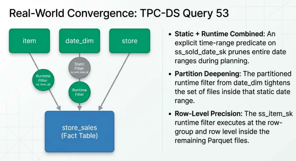
In a physical plan from a production-like run, Dremio chooses the three dimensions as build sides and store_sales as the probe side. Two of the hash joins produce runtime filters that are consumed by the store_sales data-file scan:

• A regular runtime filter on ss_item_sk, derived from the filtered item dimension.
• A partitioned runtime filter on ss_sold_date_sk, derived from the filtered date_dim.

At the same time, the query has an explicit time-range predicate on ss_sold_date_sk (a standard partition filter). That static predicate prunes away whole date ranges up front. The partitioned runtime filter further tightens the set of partitions and files within that range, while the ss_item_sk filter works primarily at the row-group and row level inside the remaining files.

The key takeaway is that runtime filters layer on top of your existing pruning:

• Static predicates (like the time window on ss_sold_date_sk) and partitioning get you the big, predictable wins.
• Runtime filters then adapt to the actual keys produced on the build side for this specific query run, trimming away even more of the fact table that could never participate in the join.

When Runtime Filters Help (and When They Don't)

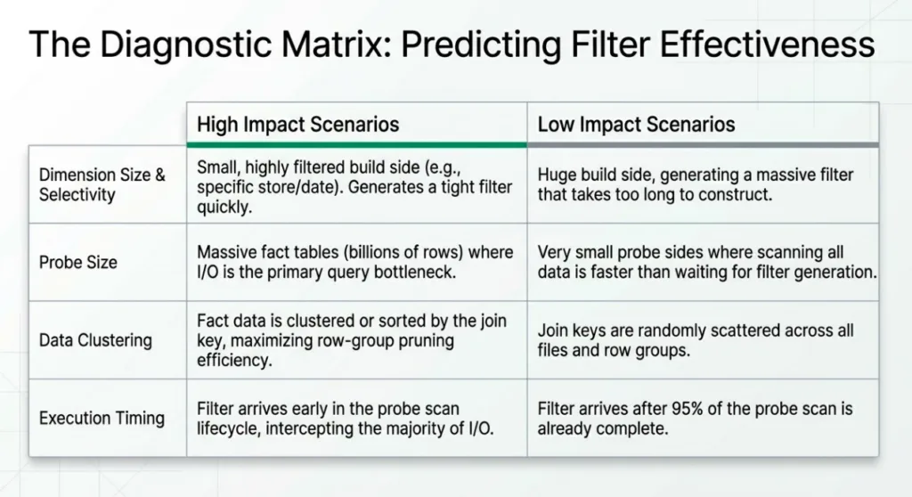
Runtime filters shine in some patterns and are barely noticeable in others. You can think about their effectiveness in terms of size, shape, and timing.

Cases where runtime filters help a lot

• Large fact-table probe, small selective dimensions (like TPC-DS q53)
  This is the most effective pattern: a big Parquet/Iceberg fact table such as store_sales on the probe side, joined to smaller dimensions (item, date_dim, store) with selective predicates. The build sides see a relatively small set of join keys, so the runtime filter is tight and can aggressively prune partitions, files, and row groups on the probe side.
• Equi-joins on well-behaved keys
  Runtime filters are designed around equi-joins on keys. When you join on clean key columns (e.g., ss_item_sk = i_item_sk, ss_sold_date_sk = d_date_sk), Dremio can efficiently collect keys on the build side and apply them on the probe side. Expression-based joins (f(key) = other_key) or non-equi joins (ranges, inequalities) are much harder to turn into effective runtime filters.
• Keys aligned with layout and metadata
  Filters are most powerful when the join keys line up with how the data is laid out:
  • The key (or a correlated key) is part of the partition spec.
  • The key has good row-group statistics and Bloom filters. In those cases, runtime filters can drop entire partitions/files and skip many row groups, saving both I/O and CPU.
• Queries that run long enough for filters to arrive early relative to the probe
  On large fact scans like our q53 example, the probe side runs long enough that even filters produced partway through the query still arrive early enough to control almost all of the expensive work. In practice, only a small fraction of output rows tend to be emitted before the runtime filters arrive; most of the scan runs with filters active.

Cases where runtime filters help less (or not at all)

• Small probes or short-running queries
  If the probe-side input is small or the query finishes quickly, the runtime filter may be ready only after most of the probe work is already done. The overhead of constructing and shipping the filter is low, but there is simply not much work left for it to save.
• Joins that can't produce good filters
  Non-equi joins, highly complex join conditions, or joins on expressions may not yield a usable runtime filter at all. In those cases, you will not see runtime filters in the plan or profile, and other optimizations (like partition pruning and reflections) carry the load.
• Keys that don't line up with layout
  If you join on a column that is neither part of the partition spec nor well-covered by row-group metadata, a runtime filter may still act as a row-level predicate, but it cannot drop many files or row groups. You may see some CPU savings in the join, but the I/O savings will be limited.
• Heavily skewed keys
  When most of the rows share a few very popular key values, a runtime filter does not narrow things down much: almost every partition, file, or row group still contains at least one matching key. In that case, the filter is technically present but has little effect on pruning.

In practice, you get the best returns when you consciously design schemas and queries so that:

• Big fact tables are on the probe side.
• Dimensions with selective predicates sit on the build side.
• Join keys are stable, equi-joinable columns that align with partitioning and statistics.

Observability: Seeing Runtime Filters at Work

Most of the time, you'll observe runtime filters through Dremio's query profile using two views:

• The Visual Profile tab, which shows a graphical operator tree with per-node sidebars.
• The Raw Profile tab, which opens a modal with detailed tables and the final physical plan (often called the Profile Inspector).

There are two main questions to answer:

1. Did this query actually produce and consume runtime filters?
2. Did they materially reduce the amount of data scanned or processed?

1. Quick signals in Visual Profile

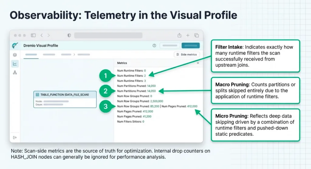
In the Visual Profile tab, selecting an operator shows a sidebar with runtime and statistics metrics.

For TABLE_FUNCTION nodes that correspond to fact-table scans (for example, a DATA_FILE_SCAN on store_sales), the most relevant metrics for runtime filters are:

• Num Runtime Filters
• Num Partitions Pruned
• Num Row Groups Pruned
• Num Pages Pruned

These give you a quick sense of whether runtime filters were active and whether pruning was significant. Num Runtime Filters tells you how many runtime filters the scan actually received from upstream joins. Num Partitions Pruned counts partitions or splits that were skipped because of runtime filters. Num Row Groups Pruned and Num Pages Pruned are more general: they include pruning driven by both runtime filters and static predicates (for example, pushed-down filters or partition filters) that were turned into Parquet/Iceberg filters.

For HASH_JOIN nodes, Visual Profile also shows join-side metrics like Runtime Filter Count and Runtime Column Count. These are mostly internal drop counters for filters that were not used (for example, because they were too large or incompatible with a scan) and can usually be ignored; for performance analysis, you'll get more value from the scan-side metrics above.

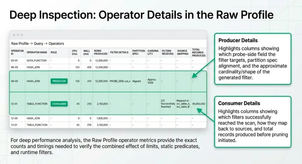
2. Detailed view in Raw Profile → Query → Operators

For deeper analysis, open the Raw Profile tab and focus on the Query → Operators section:

• The Operators overview table lists all operators by an ID of the form phaseId-xx-operatorId (for example, 02-xx-05).
• Expanding an operator shows a per-fragment table, followed by two folds:
  • Operator Details
  • Operator Metrics

For hash joins (producers), Operator Details typically includes columns such as:

• Probe Target
• Is Partitioned Column / Is Non Partitioned Column
• Probe Field Name
• (Approx) Number Of Values
• Number Of Hashfunctions

These fields describe which probe-side field the runtime filter targets, whether that field is part of the partition spec, and the approximate cardinality and shape of the filter.

For table functions / scans (consumers), Operator Details may include columns such as:

• Minor Fragment Id
• Join Source
• Is Partitioned Column
• Probe Field Name
• (Approx) Number Of Values
• Number Of Hashfunctions
• Output Records Before Pruning
• Is Dropped
• plus file/IO fields like FilePath, IO Time (ns), IO Size, Offset, Operation Type

This is where you can see which runtime filters reached a given scan, how they map back to join sources, and how many records were produced before pruning started.

Operator Metrics complements this with scan-level counters (for example, partitions/row groups/pages pruned, runtime filter counts) and timings. As in Visual Profile, these counts reflect the combined effect of static predicates, limits, and runtime filters.

3. Mapping producers to consumers via the plan

To connect specific join producers to scan consumers, you can use the Planning → Final Physical Transformation section in the Raw Profile. This is a textual representation of the final physical plan. In that text:

• Look for runtimeFilterId= on hash join operators (filter producers).
• Look for runtimeFilters= on table function / scan operators (filter consumers).

Those snippets include the same operator IDs you see in the Operators table, so you can:

1. Identify which joins produced which filter IDs.
2. Identify which scans consumed those filters.
3. Jump back to Query → Operators and open Operator Details / Operator Metrics for those specific operators.

In a query like q53, this lets you tie together:

• Hash joins on item and date_dim as producers of filters on ss_item_sk and ss_sold_date_sk.
• The store_sales scan as a consumer of both filters, with corresponding prune counts and record statistics.

4. Reasoning about effectiveness

Even without reconstructing a full timing diagram, the profile gives you useful signals about whether runtime filters are doing meaningful work:

• Pruning metrics on scans
  Compare the number of partitions/files/row groups scanned versus pruned on the fact-table scans. A high prune ratio is a strong indicator that static predicates and runtime filters together are reducing I/O.
• Scan vs join work
  Look at how much time and how many records are spent in the fact-table scan vs. the downstream join operators. If runtime filters are effective, you should see fewer records flowing into the joins and, often, reduced time spent in the scan itself.
• Before/after comparisons
  For performance investigations, comparing profiles between two runs of the same query (for example, with and without a particular dimension filter) can make the impact of runtime filters very clear. You should see differences in:
  • Partitions/files/row groups pruned.
  • Records read from the fact table.
  • End-to-end query time.

5. Going deeper (advanced analysis)

The kind of timing breakdown shown earlier in this post—for example, that runtime filters arrived after the probe became productive but still before 99.7% of the work—comes from deeper inspection of the query profile than the default UI exposes. Internally, each operator records detailed timing and runtime-filter metadata that can be analyzed offline.

For most users, the combination of Visual Profile and Raw Profile is enough to answer:

• Whether runtime filters were present at all.
• Which joins produced them and which scans consumed them.
• Roughly how much data was pruned.

When you need to debug subtle timing effects or investigate complex workloads, you (or your support team) can export the profile and use more specialized tools to reconstruct filter-generation and arrival timelines from the underlying metadata.

Practical Guidance and Best Practices

This section pulls the earlier concepts into concrete guidance you can apply when modeling data, designing queries, and reading profiles.

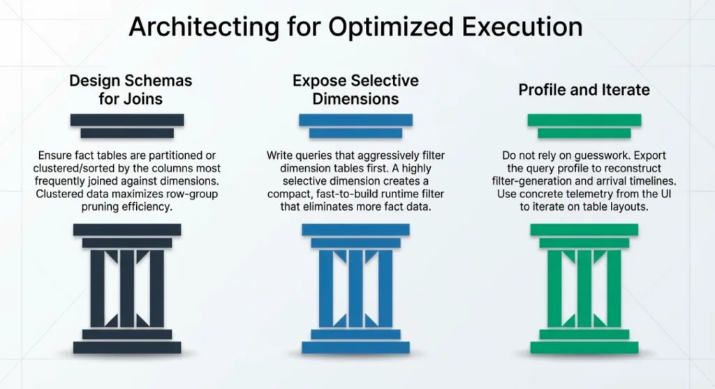
1. Design schemas and layouts with joins in mind

• Put large facts on the probe side, dimensions on the build side.
  This is the default for star schemas in Dremio, but it is worth double‑checking when you see unexpectedly large build sides in the profile. If a fact table sneaks onto the build side of a join, runtime filters will not help you much.
• Partition facts by time or other dominant filters.
  Time‑based partitioning (as in TPC‑DS store_sales on ss_sold_date_sk) combines extremely well with runtime filters from date dimensions. Partitioning on other high‑cardinality join keys is usually less effective than on time, but strong correlations (for example, regional keys for region‑scoped workloads) can still work.
• Exploit Parquet/Iceberg metadata.
  Runtime filters are most powerful when they can drive Parquet row‑group pruning and Iceberg data‑file pruning. Make sure key columns and correlated predicates have good statistics and Bloom filters; avoid writing files that are too small or too wide to accumulate useful metadata.

2. Write queries that expose selective dimensions

• Filter on dimensions, not directly on the fact.
  Instead of hard‑coding predicates on fact columns, prefer filtering on small dimensions (for example, item or date_dim) and letting joins + runtime filters push that selectivity down into fact scans.
• Use equi‑joins on stable keys where possible.
  Join on well‑behaved surrogate keys (*_sk) rather than on complex expressions. If you must join on expressions or ranges, consider whether a separate pre‑computed dimension table could hold that logic and expose a clean key join for the main query.
• Keep predicates sargable.
  Avoid wrapping join keys in functions that prevent the optimizer from using indexes and metadata (for example, cast, substr, or arbitrary UDFs on the key). Put such transformations on the non‑key side of the comparison where possible.

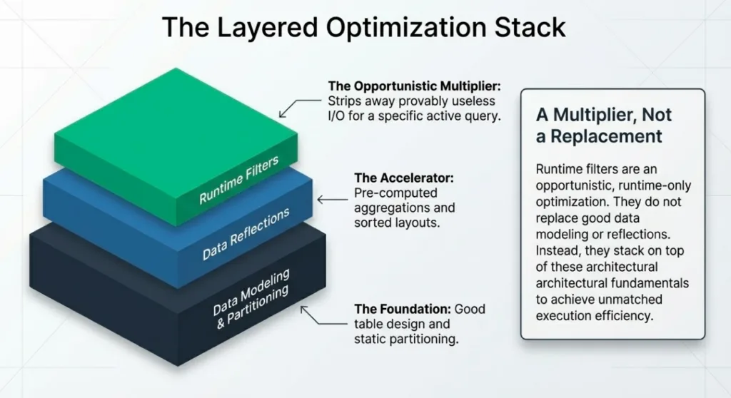
3. Combine runtime filters with reflections

• Use reflections to shorten both build and probe paths.
  Aggregation and raw reflections can pre‑cluster or pre‑aggregate data in ways that reduce the cost of both building runtime filters and scanning fact tables. From a query‑tuning perspective, reflections and runtime filters are complementary: reflections change what you scan; runtime filters change how much of that data you actually need.
• Validate that reflections preserve join keys.
  When using reflections for star‑schema workloads, ensure that the join keys used in runtime filters (for example, the surrogate keys into store_sales) remain available in the reflected data. If a reflection drops or radically transforms those keys, runtime filters may become less effective on that path.

4. Use the profile to iterate

• Start with pruning metrics.
  For slow queries, begin by inspecting fact‑table scans in the profile: are you pruning many partitions/files/row groups, or scanning almost everything? If pruning is low, focus first on schema and partitioning; if pruning is high, runtime filters and query structure are probably already pulling their weight.
• Confirm who produced and consumed filters.
  Use the Operators table and Operator Details to map producer joins (runtimefilterDetailsInfos) to consumer scans (runtimefilterDetailsInfosInScan). This gives you a concrete picture of which parts of the plan are benefiting from runtime filters.
• Make controlled changes.
  When experimenting with schema changes, reflections, or query rewrites, change one variable at a time and compare profiles. Look for differences in build‑side cardinalities, prune counts, and scan record counts to see whether runtime filters have become tighter or looser.

Conclusion and Further Reading

Runtime filters in Dremio are an opportunistic, runtime‑only optimization: they do not replace good data modeling, partitioning, or reflections, but they stack on top of those fundamentals to remove work that is provably useless for a specific query run.

The TPC‑DS q53 example shows this in a realistic setting:

• Static predicates and partitioning narrow the search space up front.
• Joins on selective dimensions generate runtime filters that further prune partitions, files, and row groups.
• Even when filters arrive after the probe becomes productive, they can still cover the vast majority of the expensive work.

If you are tuning workloads in Dremio, it is worth treating runtime filters as part of the normal toolkit:

• Design schemas and partitioning so that join keys (or correlated keys) align with layout and metadata.
• Write queries that express selectivity on small dimensions and use clean equi‑joins on keys.
• Use reflections to shorten I/O paths, and profiles to validate where runtime filters appear and how much they prune.

From there, you can iterate with concrete evidence from query profiles instead of relying on guesswork.

For further reading on related topics in Dremio, see:

• Engineering posts on reflection recommendations and intelligent reflection refresh, which focus on choosing and maintaining the right physical representations of your data.
• Deep dives into Iceberg and Parquet pruning, which explain how Dremio uses table and file‑level metadata to avoid scanning unneeded data.
• Product documentation on query profiles, reflections, and query tuning, which provides up‑to‑date details on the UI and configuration options discussed here.

Taken together, these resources give you a framework for thinking about end‑to‑end performance: from how data is laid out on disk, to how Dremio chooses plans, to how runtime filters help those plans skip work at execution time.