oct 14 – nov 13, 2025
Paris / Nuremberg / London / San Francisco / New York City


Oct 14

Oct 16

Oct 29

Nov 6

Nov 13
Saved the date
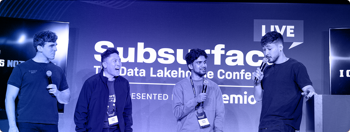
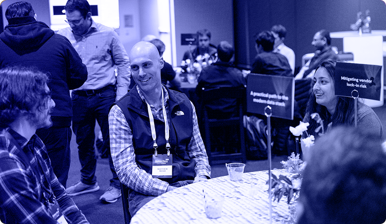
Subsurface, proudly presented by Dremio, is back—and bigger than ever.
This year’s event shines a spotlight on the latest innovations in the open data lakehouse ecosystem, with real-world use cases that bring technical depth and practical insights together. Subsurface is the global stage for data pioneers, blending cutting-edge research with hybrid lakehouse strategies that are shaping the future of data.
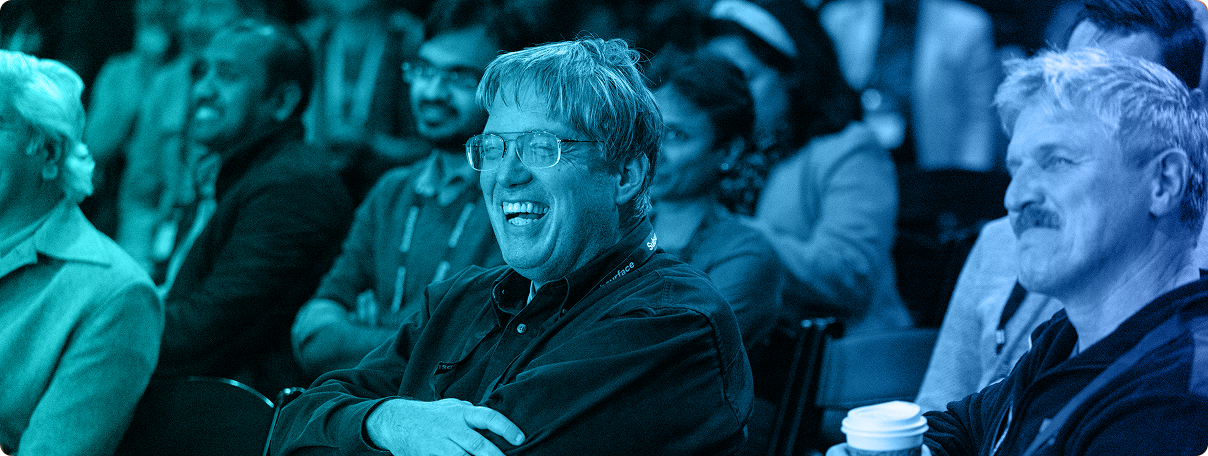
Over 18,000 data engineers, architects, and scientists from around the world have joined us at past events. Our speaker lineup has included experts from industry leaders like Apple, Netflix, Lyft, LinkedIn, TransUnion, Uber, Marsh McLennan, Adobe, AWS, Microsoft, Shell, and Wayfair—as well as emerging players like SpiceAI and Forcemetrics. We've also featured the original creators behind Apache Arrow, Apache Iceberg, Apache Parquet, Project Nessie, Pandas, and more.
This year, we’re bringing even more Dremio-focused sessions—offering a closer look at its architecture, performance gains, and role in the modern data stack.
Best of all, it’s free—and coming to a city near you. Don’t miss your chance to connect with peers, learn from industry leaders, and be part of the future of data.
Tuesday, october 14
Thurday, october 16
Wednesday, october 29
Wednesday, November 6
Wednesday, November 13
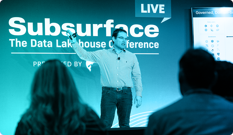
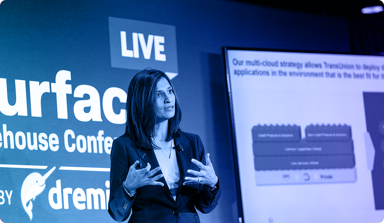
Check out some of our past speakers!


We’ve opened the call for presenters, and we’re looking for members of the data lake community to share their experience and expertise building modern cloud data lakes as well as key open source technologies such as Apache Iceberg, Apache Arrow, Apache Spark, and more.
If you have an interesting story to tell, whether it’s a success or a failure you learned an important lesson from, sharing your experience can have a real impact on the community then click below to submit a talk.
Call for speakers closes on Friday, August 15 at 11:59pm PT!
For more information on sponsorship at Subsurface LIVE 2025, please contact our Sponsorship Management Team.