The Life of a Read Query for Apache Iceberg Tables

Apache Iceberg is an open data lakehouse table format that provides your data lake with amazing features like time travel, ACID transaction, partition evolution, schema evolution, and more. You can read this article and watch this video to learn more about the architecture of Apache Iceberg. This current article aims to explain how read queries work for Apache Iceberg.
In order to understand how read queries work you first need to understand the metadata structure of Apache Iceberg, and then examine step by step how that structure is used by query engines to plan and execute the query.
Apache Iceberg 101
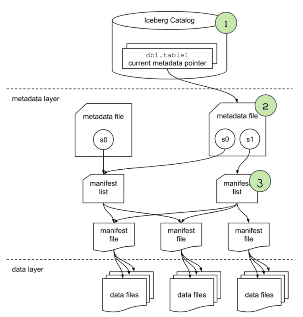
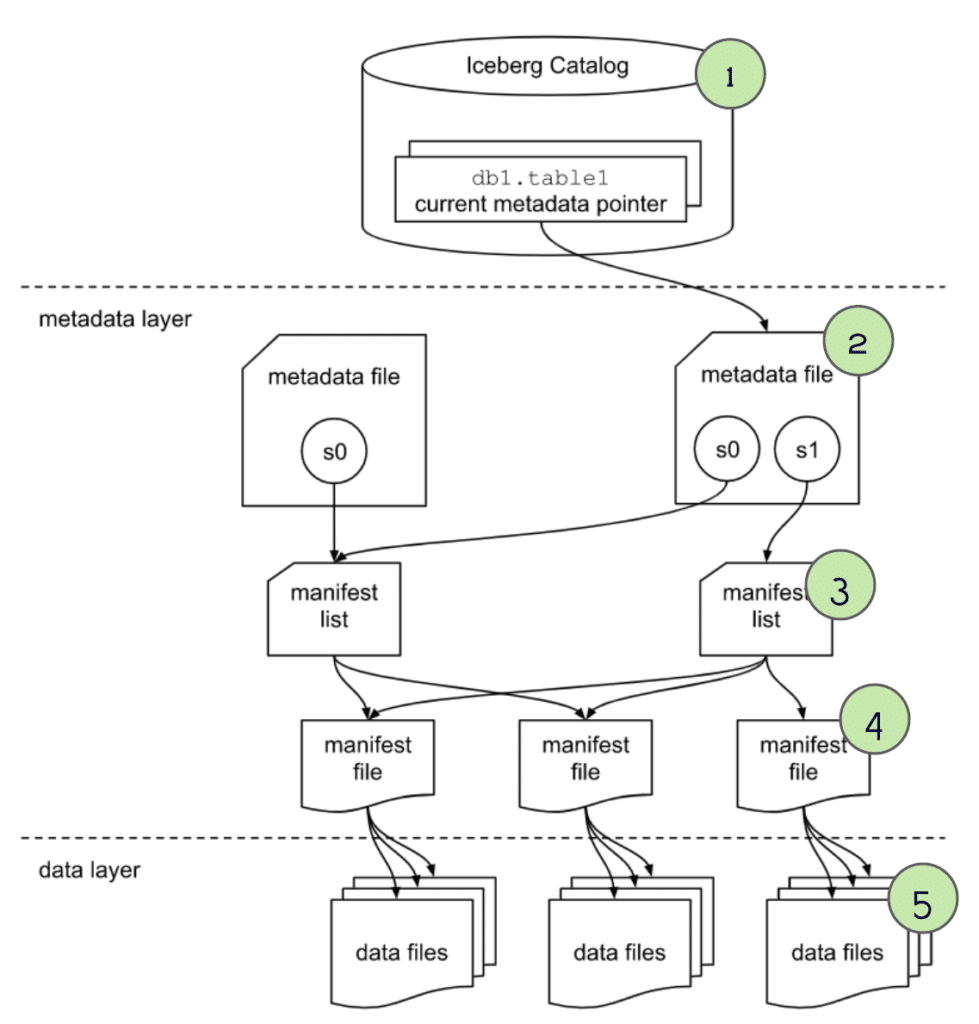
Apache Iceberg has a tiered metadata structure, which is key to how Iceberg provides high-speed queries for both reads and writes. Let’s summarize the structure of Apache Iceberg to see how this works. If you are already familiar with Iceberg’s architecture, you can skip ahead to the section titled "How a Query Engine Processes the Query."
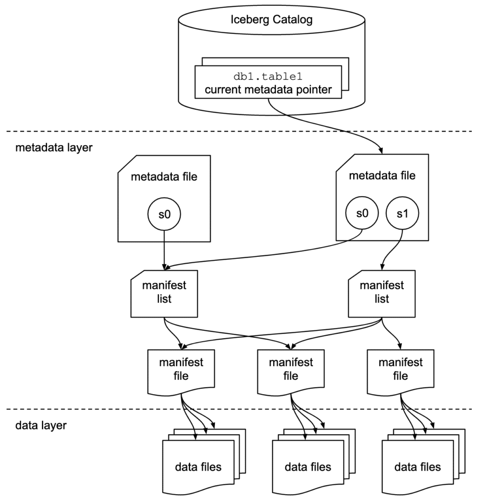
Data Layer
Starting from the bottom of the diagram, the data layer holds the actual data in the table. It’s made up of two types of files:
Data files – Stores the data in file formats such as Parquet or ORC
Delete files – Tracks records that still exist in the data files, but that should be considered as deleted
Metadata Layer
Apache Iceberg uses three tiers of metadata files which cover three different scopes:
Manifest files – A subset of the snapshot, these files track the individual files in the data layer in that subset along with metadata for further pruning
Manifest lists – Defines a snapshot of the table and lists all the manifest files that make up that snapshot with metadata on those manifest files for pruning
Metadata files – Defines the table, and tracks manifest lists, current and previous snapshots, schemas, and partition schemes.
The Catalog
Tracks a reference/pointer to the current metadata file. This is usually some store that can provide some transactional guarantees like a relational database (Postgres, etc.) or metastore (Hive, Project Nessie, Glue).
How a Query Engine Processes the Query
Running a SELECT on the table’s current state
We are working with a table called “orders” which is partitioned by the year of when the order occurred.
If you want to understand how a table like the orders table was created and has data in it, read our post on the life of a write query for Iceberg tables.
CREATE TABLE orders (...)
PARTITIONED BY (year(order_ts));
Let’s run the following query:
SELECT *
FROM orders
WHERE order_ts
BETWEEN '2021-06-01 10:00:00' and '2021-06-30 10:00:00';
1. The query and the engine
The query is submitted to the query engine that parses the query. The engine now needs the table’s metadata to begin planning the query.
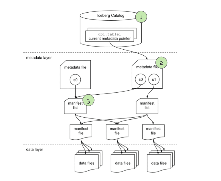
2. The engine gets info from the catalog
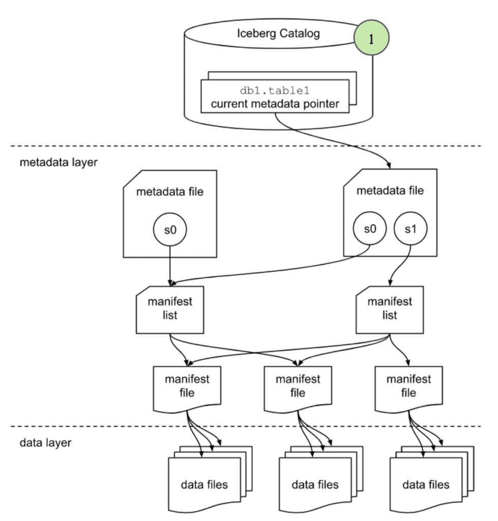
The engine first reaches out to the catalog and asks for the file path of the orders table’s current metadata file.
3. The engine gets info from the metadata file
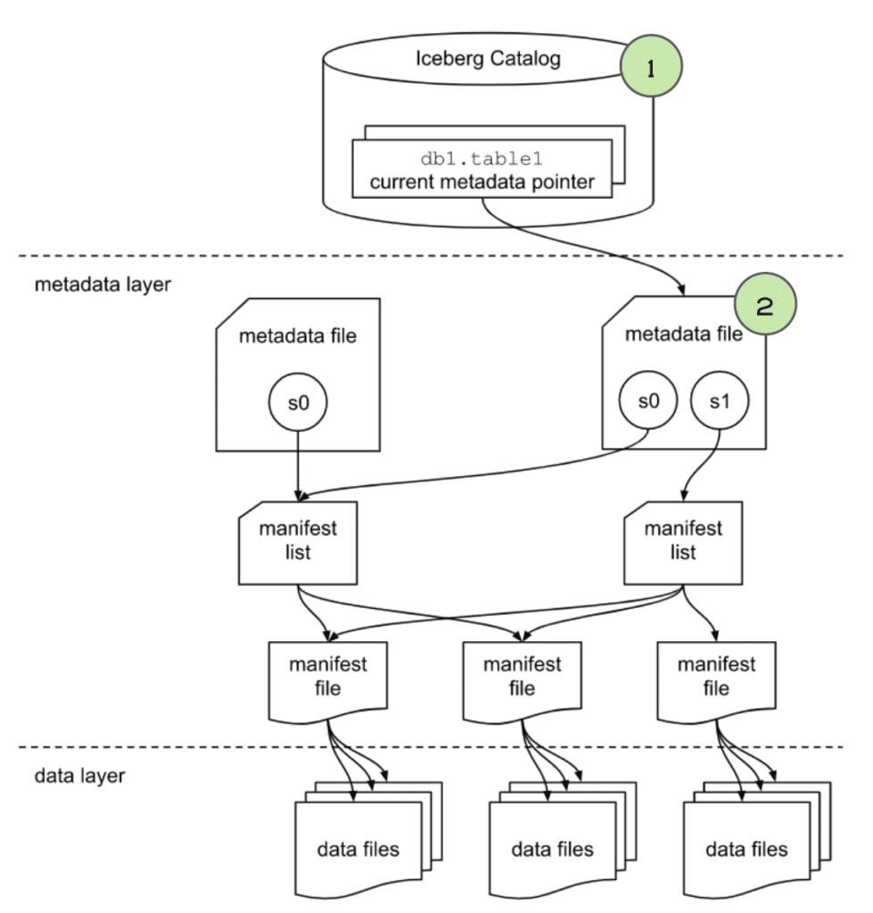
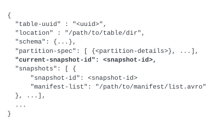
The engine uses the orders table’s latest metadata file to determine a few things:
- The table's schema.
- The partitioning of the table to determine how the data is organized so it can prune files later in query planning that aren’t relevant to our query.
- The current snapshot’s “Manifest List” file so it can determine what file to scan.
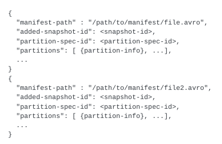
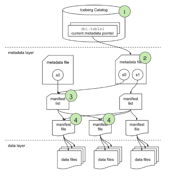
4. The engine gets info from the manifest list file
The “manifest list” file lists several useful pieces of information we can use to begin planning what files should be scanned. Primarily, it lists several “manifest” files which each have a list of data files that make up the data in this snapshot. The engine will primarily look at:
- The
partition-spec-id, so it knows, together with partition spec info from the metadata file, what partition scheme was used for writing this snapshot. For this table, thepartition-spec-idwould be 0 since it only has one partition spec (Partitioned by year oforder_ts).
- The partition field summaries, which includes data on partition columns within each manifest which contain the upper and lower bounds of partition fields in the manifest. This can be used to determine whether a manifest can be skipped or scanned to evaluate the individual data files in it. So in our case, any manifest that doesn’t contain
order_tsvalues in2021can be pruned. This process will be repeated more granularly against individual files when we analyze the individual manifests in the next step.
This is where we can see huge query planning and execution gains. Instead of pruning data files one by one, we can eliminate large groups of files by eliminating unneeded manifests.
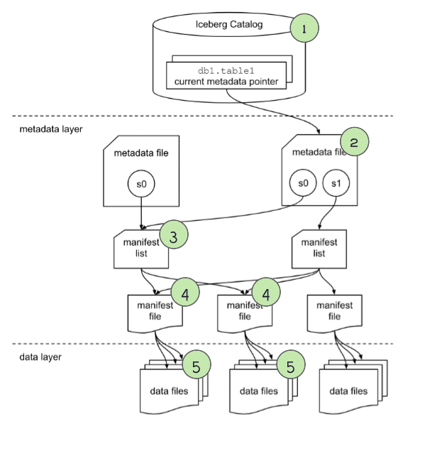
5. The engine gets info from the manifest files
For any manifest files that weren’t pruned when scanning the “manifest list” we then scan each of those manifest files to find a list of individual data files with useful metadata on each file:
- The
schema-idandpartition-idfor the data file. - The type of content, i.e., whether it is a data file with records or a delete file with a specification of records to be deleted/ignored.
- Counts of values, unique values, and the upper and lower bounds for each column that is being tracked (stats tracking for individual columns can be adjusted in table settings). So in this case it can use the upper/lower bound values to eliminate any files that contain no records in June 2021, that way we only scan data files that have relevant data.
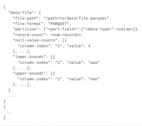
These column stats can be used to determine if a data file is relevant to this query, and prune it from scanning if it isn’t, which will speed up query execution.
Performing the Scan and Returning the Results
At this point, we have the narrowest possible list of data files that need to be scanned. The query engine now begins scanning the files and doing any remaining processing requested by the query to get the final result.
This query will be significantly faster than a full table scan because thanks to the partitioning and min/max filtering during query planning we can scan a much smaller subset of the full table.
If this were a Hive table we would’ve seen this play out differently in a few ways:
- There would’ve been a lot more file operations without the pruning at the metadata level, making for a longer more expensive query.
- We couldn’t have benefited from Iceberg’s Hidden Partitioning and would’ve needed to create a separate partition column (
order_year) that would have also needed to be explicitly filtered to avoid a full table scan, which users often don’t do.
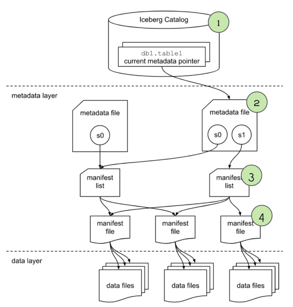
Running a Read on the Table’s Current State After the Partitioning Has Evolved
So let’s run another query against the orders table. Let’s assume the following:
- The table was initially partitioned based on year (
PARTITIONED BY (year(order_ts))) up until 2021, but starting January 1, 2022, the table was changed to partition by both year and day (ADD PARTITION FIELD day(order_ts)).
Let’s run the following query:
SELECT *
FROM orders
WHERE order_ts BETWEEN '2021-06-01 10:00:00' and '2022-05-3110:00:00';
1. The query and the engine
The query is submitted to the query engine that parses the query. The engine now needs the table’s metadata to begin planning the query.
2. The engine gets info from the catalog
The engine first reaches out to the catalog and asks for the file path of the orders table’s current metadata file.
3. The engine gets info from the metadata file
The engine uses the orders table’s latest metadata file to determine a few things:
- The table's schema.
- The partitioning of the table to determine how the data is organized so it can prune files later in query planning that aren’t relevant to our query.
- The current snapshot’s “Manifest List” file so it can determine what file to scan.
4. The engine gets info from the manifest list file
The “manifest list” file lists several useful pieces of information we can use to begin planning what files should be scanned. Primarily, it lists several “manifest” files which each have a list of data files that make up the data in this snapshot. The engine will primarily look at:
- The
partition-spec-id, so it knows, together with partition spec info from the metadata file, what partition scheme was used for writing this snapshot. For this table, thepartition-specwas evolved so files written after the partitioning spec was changed would have apartition-spec-idof1(partitioned by year and day) versus files that were written before the partitioning spec was changed, which would have apartition-spec-idof0(partitioned by year only).
- The partition field summaries, which includes data on partition columns within each manifest which contain the upper and lower bounds of partition fields in the manifest. This can be used to determine whether a manifest can be skipped or scanned to evaluate the individual data files in it. So in our case, any manifest that doesn’t contain data files that have
order_tsvalues in 2021 or in the first 5 months of 2022 can be pruned. This process is split based on partitioning spec, so manifests based onpartition-spec-id0 will be pruned based on the original partitioning and the manifests based onpartition-spec-id1 will be pruned based on the newer partitioning scheme. This process will be repeated against individual files when we analyze the individual manifests in the next step.
This is where we can see huge query planning and execution gains. Instead of pruning data files one by one, we can eliminate large groups of files by eliminating unneeded manifests.
5. The engine gets info from the manifest files
For any manifest files that weren’t pruned when scanning the “manifest list” we then scan the manifest to find a list of individual data files with useful metadata on each file:
- The
schema-idandpartition-idfor the data file. - The type of content, whether it is a data file with records or a delete file with a specification of records to be deleted/ignored.
- Counts of values, unique values, and the upper and lower bounds for each column being tracked (stats tracking for individual columns can be adjusted in table settings). So in this case it can use the upper/lower bound values to eliminate any files that contain no records between June 2021 and May 2022. That way we only scan data files that have relevant data.
These column stats can be used to determine if a data file is relevant to this query, and prune it from scanning if it isn’t, which will speed up query execution.
Performing the Scan and Returning the Results
Now we have the narrowest possible list of data files that need to be scanned. The query engine now begins scanning the files and doing any remaining processing requested by the query to get the final result.
This query will be significantly faster than a full table scan because thanks to partitioning and min/max filtering during query planning we can scan a much smaller subset of the full table.
Running a SELECT on a previous state of the table
Run the following query:
SELECT *
FROM orders TIMESTAMP AS OF '2022-06-01 10:00:00'
WHERE order_ts BETWEEN '2021-06-01 10:00:00' and '2022-05-31 10:00:00';
Notice, this TIMESTAMP AS OF specifies a desire to time travel using the AS OF clause, stating we want to query the table’s data as it existed on June 1, 2022 at 10 am.
The query and the engine
The query is submitted to the query engine that parses the query. The engine now needs the table data to begin planning the query.
Checking the catalog
The engine first reaches out to the catalog and asks for the file path of the orders table’s current metadata file.
Checking the metadata file
With the latest metadata file, the engine can determine a few things:
- The desired snapshot, starting with the current snapshot and comparing the snapshot ID or snapshot timestamp to the
AS OFclause until the snapshot that was current at that point in time is found. - The table's schema.
- The partitioning of the table to determine how the data is organized so it can later prune files that aren’t relevant to our query.
- The target snapshot’s “Manifest List” file so it can begin to determine what file to scan.
Checking the snapshot
The “manifest list” file lists several useful pieces of information we can use to begin planning what files should be scanned. Primarily, it lists several “manifest” files which each have a list of data files that make up the data in this snapshot. The engine will primarily look at:
- The
partition-spec-id, so it knows what partition scheme was used for writing this snapshot. - The partition field summaries, which includes data on partition columns within each manifest which contain the upper and lower bounds of partition fields in the manifest. This can be used to determine whether a manifest can be skipped or scanned to evaluate the individual data files in it.
This is where we can see huge query planning and execution gains because instead of pruning data files one by one, we can eliminate groups of files by eliminating unneeded manifests.
Checking the manifests
For any manifest files that weren’t pruned when scanning the “manifest list” we then scan the manifest to find a list of individual data files with useful metadata on each file:
- The
schema-idandpartition-idfor the data file. - The type of content, i.e., whether a data file with records or a delete file with a specification of records to be deleted/ignored.
- Counts of values, unique values, and the upper and lower bounds for each column that is being tracked (stats tracking for individual columns can be adjusted in table settings).
These column stats can be used to determine if a data file is relevant to this query, and prune it from scanning if it isn’t, which will speed up query execution.
Performing the scan and returning the results
Now we have the narrowest possible list of data files that need to be scanned. The query engine now begins scanning the files and applying any filters to get the final result. This query will be vastly faster than a full table scan because thanks to partitioning and min/max filtering during query planning we can scan a much smaller subset of the full table.
Conclusion
Apache Iceberg, using its metadata, can help engines execute queries quickly and efficiently on even the largest datasets. Beyond the partitioning and min/max filtering, we illustrated in this article, we also could have optimized the table even further by sorting, compacting, and other performance practices.
Apache Iceberg provides the flexibility, scalability, and performance your modern data lakehouse requires.
Get a Free Early Release Copy of "Apache Iceberg: The Definitive Guide".
About the Author
Alex Merced
Alex Merced is a developer advocate for Dremio and has worked as a developer and instructor for companies like GenEd Systems, Crossfield Digital, CampusGuard and General Assembly. Alex is passionate about technology and has put out tech content on outlets such as blogs, videos and his podcasts Datanation and Web Dev 101. Alex Merced has contributed a variety of libraries in the Javascript & Python worlds including SencilloDB, CoquitoJS, dremio-simple-query and more.
Related Articles
Compaction in Apache Iceberg: Fine-Tuning Your Iceberg Table’s Data Files
Read more
Puffins and Icebergs: Additional Stats for Apache Iceberg Tables
Read more